1. Prospectus & Regression I
Introduction
Phil Donoghue, the editor of this publication, recently wrote to inquire whether I would be interested in writing a regular column on quantitative data-analysis techniques for palaeontologists. My first reactions were amusement, concern, and then fear, in that order. Amusement because, as a field, palaeontology is no slouch when it comes to assimilating new quantitative methods. Among practitioners of the natural sciences, palaeontologists have often been among the first to employ new data analysis methods in innovative applied contexts (e.g., factor analysis, Monte Carlo simulation, bootstrapping, morphometrics) and our ranks boast several individuals who have played prominent roles in the development and popularization of both semi-quantitative and fully quantitative techniques (e.g., Imbrie, Reyment, Shaw, Raup, Marcus, Gould). Concern because palaeontologists also have a well-deserved reputation of being sceptical of mathematical results and generally don’t conceive of their science as being mathematical. Far too often have I heard talented practitioners cite an antipathy toward mathematics as the reason they opted for the geosciences in the first place and palaeontology in particular. Indeed, I recall vividly the time when, at my first Geological Society of America meeting, after having spent some time patiently explaining my poster dealing with a morphometric analysis of radiolarian evolution, one of the grand old men of American palaeontology congratulated my advisor for having secured the skills of a young palaeontologist who ‘can really make those numbers dance’. How can I hope to persuade a group that as made an overall indifference to numerical methods a point, not only of pride, but the imprimatur of a kind of folk wisdom, that numbers aren’t only useful, but beautiful and fun. Which leads me to fear. The fact is, with each passing year science becomes more quantitative. This should be welcomed. Quantification has been the hallmark of a maturing science ever since Descartes and Newton. Even the qualitative bastion of taxonomy will soon feel its effects in much the same way phylogenetic analysis did some two decades ago. But there is also danger here. As the tools of quantitative analysis become easier to use, and are employed more frequently, my experience has been that understanding of the fundamentals of numerical analysis becomes ever more important. Those who don’t understand the difference between parametric non-parametric approaches, correlation and covariance, and relative and principal warps not only put themselves at a disadvantage in examining their own data, they quickly surrender their ability to make informed decisions about the increasingly large number of studies that apply—or, in many cases, mis-apply—such methods. Taking responsibility for guiding a traditionally reluctant audience through such material, separating its core truths from the aficionado’s love of detail, and providing it but with a practical understanding they can use to come to their own conclusions about their own data, is daunting task. But that’s what’s needed and that’s what I will try to provide.
In each essay I’ll try to illuminate a corner of quantitative method and practice with an emphasis on practicality in a palaeontological context. These articles will not be written for specialists in quantitative analysis. Those with such experience should already be aware of much of the material I intend to present, though I will try to juxtapose topics in novel and hopefully appealing ways. Rather, they will be written for those who always wanted to gain knowledge of this subject, but never had the opportunity to do so and haven’t managed to make much progress through self-education. In addition, I’ll try to illustrate the methods discussed with spreadsheets containing the various formulas and procedures rendered in a form acceptable to that indispensable piece of data-analysis software sitting on your computer desktops right now; the venerable MS-Excel. On occasions where the method exceeds Excel’s abilities, I’ll point you to inexpensive software you can use to perform the procedure.
But you must play your role too. If, in an essay I say or do something you don’t understand, please tell me. If there’s some data analysis problem you’re having and are stuck for a solution, please suggest it as a topic for a future article. Most of all, I’ll need your forbearance. To my knowledge nothing like this has been attempted in the PalAss newsletter before. It may work. It may not. Regardless, it will be interesting to find out.
Prospectus & Regression
Let us begin with two columns of numbers representing measurements of glabellar maximum length and width measurements from 18 trilobite species:
| Taxon | Length (mm) | Width (mm) | |
|---|---|---|---|
| 1 | Acaste | 5.10 | 3.46 |
| 2 | Balizoma | 4.60 | 6.53 |
| 3 | Calymene | 12.98 | 14.15 |
| 4 | Ceraurus | 7.90 | 5.32 |
| 5 | Cheirurus | 12.83 | 12.96 |
| 6 | Cybantyx | 16.41 | 13.08 |
| 7 | Cybeloides | 6.60 | 6.84 |
| 8 | Dalmanites | 10.00 | 9.12 |
| 9 | Delphion | 8.08 | 10.77 |
| 10 | Narroia | 15.67 | 9.25 |
| 11 | Ormathops | 4.53 | 4.11 |
| 12 | Phacopdina | 6.44 | 6.94 |
| 13 | Pricyclopyge | 21.53 | 14.64 |
| 14 | Ptychoparia | 12.82 | 9.36 |
| 15 | Rhenops | 22.27 | 17.56 |
| 16 | Sphaerexochus | 4.93 | 6.21 |
| 17 | Trimerus | 16.35 | 15.02 |
| 18 | Zachanthoides | 13.41 | 8.51 |
I’m going to assume, for the purposes of this initial essay, you are familiar with basic sample description indices (e.g., mean, standard deviation). These numbers describe your data and tell you things about the population from which the sample was drawn. Such parameters are used in data analysis, but they aren’t analytic results themselves.
One of the basic data analytic tools is linear regression analysis, sometime described as ‘shooting a line’ through your data. More precisely, one uses regression analysis to create a model of the manner in which one variable behaves relative to another. Such models do two basic things for the analysis. First, they provide a precise estimate of the specific relation between the variables. In a sense, you can regard this as making known that aspect of variability all objects included in the analysis have in common. Second, they provide a measure of each object’s uniqueness, in terms of its degree of deviation from the model. These two factors are expressed in the generalized equation for all linear regressions.
(1.1) yi=mxi+b+ε
In this equation, the regression line’s slope (m) expresses the aspect of between-variable behaviour that refers to the relative rates of change. Slope values of less than 0.5 (< 0.5) mean that a unit change in the x variable engenders a less than unit change in the y variable. Slope values greater than 0.5 (> 0.5) mean that a unit change in the x variable engenders a greater than unit change in the y variable. While this estimate of change rates is often the practical target of a data analysis, the slope by itself does not specify the entire model. In order to do that the position of the model in the space defined by the variables must be tacked down in such a way as to ensure that the model ‘runs through’ the data. This aspect of the model is determined by the y-intercept which is represented by the symbol b in equation 1.1. The y-intercept is a constant because it expresses the constant positional relation between the model to the data.
The third term in equation 1.1, ε represents the idea that real data deviate from the ideal. This term is left off many textbook regression equations and, aspects of the problem relating to this deviation factor are, consequently, seldom discussed. This is a great pity because the key to understanding what regression analysis is all about, and, more importantly, the key to avoiding the most common error palaeontologists make when undertaking a regression analysis, is embodied by the concept of ε.
The mathematical point of any regression analysis is to create a way of calculating the values of m and b such that, when summed over the entire sample, the total ε is minimized. Before we discuss what ‘minimized’ might mean in this context, let’s do a simple experiment. Figure 1 contains a scatterplot of the Table 1 data with each symbol representing a different genus. Without recourse to any calculations—by ‘eye’, as it were—fit a straight line to these data. Don’t worry about marring your perfect collection of Palaeontological Association Newsletters. Just get out a straight-edge and do it.
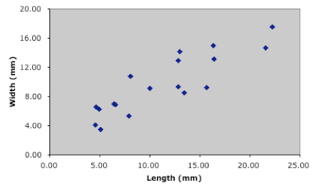
Figure 1. Scatterplot of Table 1 trilobite data.
OK. That’s your model of covariation between these two variables based on this sample of 18 trilobite glabellar measurements. We could, but won’t, determine the slope, y-intercept for your model, we could then use that to calculate a set of predicted -values based on the Table 1 x-values, and finally we could compare those predicted y-values to the measured values given in Table 1 and calculate the deviation (ε) of each point from the model. We could then compare everyone’s model across the entire Association to determine how similar each was to every other. My guess is that they would all be pretty similar. It’s a small, well-constrained data set with a clear trend. No problem.
Let’s now try a standard regression analysis of these same data produced by, say, MS-Excel. This can be done in two ways. Either you can use Excel’s ‘Paste Function’ button (fx) to find, and select the appropriate parameters for the build-in statistical SLOPE and INTERCEPT functions, or you can first plot the data as I have done in Figure 1 and then use the ‘Chart’ Pull-Down Menu’s ‘Add Trendline…’ function to specify and plot the linear regression on the chart. Either method produces the same results. Both methods are illustrated in the spreadsheet that accompanies this article. If you opt for the latter, or if you create a graphic model in another software application, your plot should look something like Figure 2.
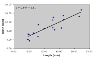
Figure 2. Regression model for the Table 1 data resulting from use of the MS-Excel default linear trendline function. The slope and y-intercept of this line are identical to those specified by Excel’s built-in statistical SLOPE and INTERCEPT functions.
Compare your linear model with Excel’s. Are they the same? Take a close look at Excel’s model. Do you believe this line is really minimizing the deviation between each data point and the linear trace of the model? I don’t. What’s going on?
When you drew your model line, what were you trying to minimize? Excel uses what has come to be the standard error-minimization strategy termed, somewhat misleadingly, ‘least-squares’ (L-S). Specifically, Excel—along with virtually all software-based regression applications—construct their model to minimize the square of the deviation of the points from the model line. Why do they use the square of the deviation instead of the raw deviation? It’s really a bookkeeping convention that avoids having to deal with negative numbers in the form of deviations from points that fall below (rather than above) the model. The L-S convention itself isn’t the problem. The reason why most L-S regressions differ systematically from ‘eyeball’ regressions is that this L-S convention is carried out over only one of the two variables (Fig. 3). Consideration of e with reference to only one variable in this way has the effect of ‘pulling’ or ‘rotating’ the regression model to a position of greater alignment with the axis over which deviation is not being minimized. If the deviation is minimized in terms of the y-variable, the regression is properly termed an ‘x on y least-squares regression’ whereas minimization over the x-variable is termed a ‘y on x least-squares regression’. Because of the asymmetry of the minimization criteria, x on y regressions will estimate models that differ from y on x regressions.
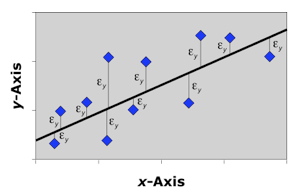
Figure 3. Error-minimization scheme used by the x on y least-squares linear regression method. Note this method only minimizes error with respect to the y-variable.
The purpose of these types of regressions is (1) prediction of a dependent variable in terms of an independent variable, (2) adjustment for a confounding variable, and (3) determination of a relation for use in assay analyses. In each case there exists a logical distinction between the two variables. One—usually the -variable—is regarded as being the subject of the analysis and the other—usually the -variable—the object of the analysis. Put another way, variation in one variable is conceived as being tied to, or best expressed as, variation in the other. Such one-dimensional least-squares regression models can also be used to test for the existence of a non-zero trend in the data and will, of course, ‘fit a line’ to a set of data. In these cases, though, the priority of an approach that minimizes e over only a single variable is open to question. After all, one can easily think of other minimization criteria that could be applied to the Table 1 data; such as the one you applied when you drew your ‘eyeball’ model.
It would be one thing if one-dimensional L-S analysis was listed as an option in regression software packages. Unfortunately, it’s not. The fact is MS-Excel, Statistica, SysStat, StatWorks, and so forth all offer x on y least-squares regression as the only programmed option for regression analyses. Indeed, in MS-Excel’s short, on-line definition of the SLOPE function, we learn that this routine ‘returns the slope of the linear regression line through the given data points’ (emphasis mine); as if x on y L-S regression was the only minimization criterion available for linear regression.
Fortunately, other regression models exist that more faithfully capture the two-dimensional geometry of data such as those included in Table 1. In most palaeontological analyses is no clear-cut need or desire to distinguish between the roles of different variables. Why should glabellar length measurements be regarded as fundamentally different from glabellar width measurements? What is to be gained from expressing e in our model only in terms of deviations on glabellar width?
One of the most useful of these alternative linear regression methods is reduced major axis (RMA) regression (Kermack and Haldane 1950; also called the relation d’allométrie, geometric mean regression, and the standard major axis). Reduced major axis regressions minimize the product of deviations from the model along both x and y axes (Fig. 4). Calculation of an RMA regression slope is unexpectedly easy, being the simple ratio between the standard deviations of variable x and variable y.
(1.2) m=sxsy
This slope also has a satisfying relation to L-S regression, being the geometric mean of the y on x and x on y regression slopes. The fact that the slope is calculated from the variable standard deviations is also useful in many (but not all) contexts insofar as this renders the regression insensitive to differences in the magnitudes of the numbers being used to represent the variables. In other words, RMA regressions can be used to compare apples and oranges (or, to be slightly more palaeontological, foraminifera and temperature, dinosaurs and rainfall, and so forth), as well as apples and apples (e.g., foraminifera and dinosaurs).
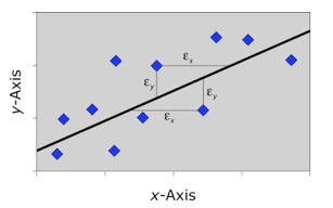
Figure 4. Error minimization scheme used by the reduced major axis regression method. This method minimizes error with respect to both x and y variables as a function of their joint product. This is equivalent to minimizing the area of the triangle formed by the projection of the data point’s x and y coordinates and the regression model.
What about the y-intercept? There’s only one standard formula for this that is used by all regression methods. It’s the projection, onto the y-axis, of a line with slope m that is constrained to pass through the bivariate mean.
(1.3) b=¯Y−m¯X
There’s one more bit to the RMA calculation. Since the value of the standard deviation is always positive, the raw ratio of standard deviations will always return a positive number, even for variables whose regression line should have a negative slope. Unlike least-squares methods, the sign of the RMA slope is determined by a separate calculation. It’s the sign of the sum of products, but not the raw sum of products.
(1.4) SP=∑xmcymc
In order to get the correct sign you’ll need to express your data in terms of each variable’s deviation from its mean.
(1.5) xmc=x−¯X
(1.6) ymc=y−¯Y
The correct answer will also be given by the corrected sum of products, but that equation is slightly more complex.
How does RMA stack up with respect to the trilobite data? Results of an RMA regression on the Table 1 data are shown in Figure 5. Compare that model to the one you drew at the start of this essay. Closer to your ‘eyeball’ estimate? Probably. When we estimate lines by eye we instinctively try to minimize error in both x and y, not with regard to just x (or just y) alone. The programmers of statistical software select L-S regressions as their default because they are trying to do right by their main audience. Least-squares models are precisely what you would want to choose in a wide variety of business and manufacturing contexts. That’s fine, even laudable. But it doesn’t mean x on y L-S regression is the best choice for everyone in every instance. In particular, L-S methods are usually, if not the wrong choice, the less-than-obvious choice for many natural history applications of regression.
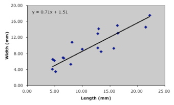
Figure 5. Regression model for the Table 1 data resulting from use of the reduced major axis regression method. Unlike, standard least-squares approaches, this model is invariant to the selection of which variable is portrayed on which axis, and to differences in variable type.
Of course, if all bivariate data points are clustered tightly around a line the difference between these two types of regression will be small. For data that have a fair amount of scatter about the trend though—and here we’re talking about most palaeontological data—the difference will be noticeable and possibly important. For the trilobite example, the angular deviation between the two regression models is only 2.5° and the conclusion that glabellar width is distributed in a linear manner, but at a lower overall rate than glabellar length, would be supported regardless of which model was accepted as correct. Nevertheless, the 'odd' trend of the LS regression is quite obvious once you look at it. Note also, this was an example calculation and we had no way of knowing the regression models would be close (but noticeably different) at the outset.
Rather than run both models on all you data to see if model choice makes a difference, why not decide which model is most appropriate to your need and use that from the start? Only used L-S regression where there is a definite causality relation between your variables and in cases where you know which direction the cause-effect arrow is pointing. If you don’t know these things, you’re better off with RMA or an alternative method I’ll discuss next time. Above all, never trust a statistics application to look out for your best interests or to give you the whole story about a method.
Further Reading
Reduced major axis regression is one of those topics that is rarely mentioned in statistical textbooks (even those who claim to be aimed at ‘scientists’) and, in those rare instances where they are mentioned, the discussion is usually incomplete. The following represent the sum total of discussions in textbooks of which I am aware, along with the original RMA reference. Caveat emptor.
DAVIS, J. C. 2002. Statistics and data analysis in geology (third edition). John Wiley and Sons, New York. 638 pp. – Contains a brief discussion of RMA regression, but neglects to mention how the sign of the RMA slope is determined. Previous editions contain no mention of RMA.
KERMACK, K. A. and HALDANE, J. B. S. 1950. Organic correlation and allometry. Biometrika 37: 30–41. – Where it all started for RMA regression.
SOKAL, R. R. and ROHLF, F. J. 1995. Biometry: the principles and practice of statistics in biological research (third edition). W. H. Freeman, New York. 887 pp. – The best discussion of non-least squares regression methods available, including RMA. Pay careful attention to their symbol conventions.
SWAN, A. R. H. and SANDILANDS, M. 1995. Introduction to geological data analysis. Blackwell Science, Oxford. 446 pp. – Very brief mention of RMA, no discussion of how to find the correct sign of the RMA regression slope.
