17. Shape Theory
Written by Norm MacLeod - The Natural History Museum, London, UK (email: n.macleod@nhm.ac.uk). This article first appeared in the Nº 71 edition of Palaeontology Newsletter.
Introduction
Now that we’ve come to grips with Procrustes superposition we’re in a position to understand what shapes really are and how they are distributed in a geometric space. From there the problems associated with analyzing shapes with traditional, distance-based variables will be obvious, as will the manner in which shapes should be analyzed. This material all falls under the general heading of ‘shape theory’ which is part of the mathematical field of topology. Even mathematicians find topology an arcane, complex and difficult subject. So, you’ll be relieved to learn we’re not going to discuss in detail. But I will need to introduce you to some basic topological concepts in the context of the discussion.
Shape Theory
Let’s begin the discussion with a simple example of the standard approach to the description of shape. Consider the set of triangles shown in Figure 1.
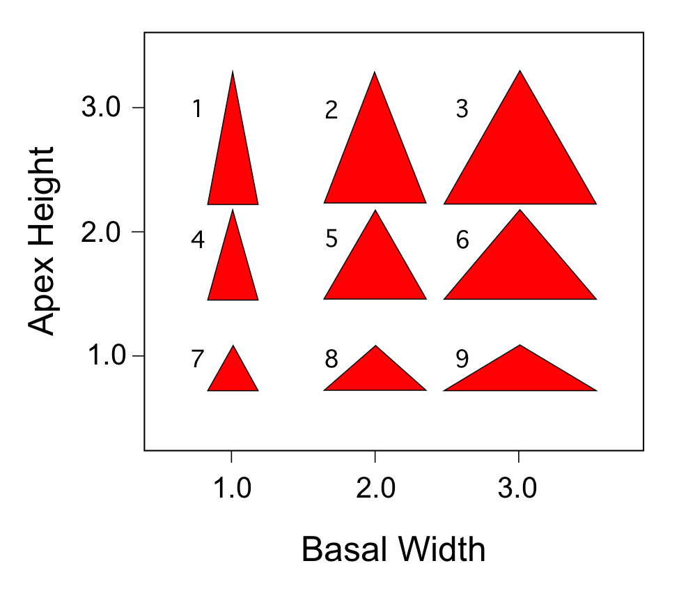
Figure 1. Nine triangles with positions plotted in a distance-based morphometric space.
The standard distance-based variables used to describe triangles are basal width and apex height.1 Note these distances make a clear distinction between the apex landmark and basal landmarks, with the latter able to be further subdivided into right and left locations. Accordingly, these variables could be calculated for any set of three landmarks used to portray the relative positions of structures on a fossil body. Indeed, this triangle measurement system assumes that each landmark can be defined uniquely within its set.
Once the landmarks have been located it is a trivial task to place each shape in its correct position relative to others in the space formed by these two variable axes. This is precisely the sort of shape space we used in our discussions of regression and multivariate data analysis. But is a space so defined fully adequate to express similarities and differences among these objects?
The first hint that this might not be the case comes through inspection of the diagonal of triangle shapes from lower left to upper right. These are all equilateral triangles (= all sides of equal length) and so have the same shape. The difference between the triangles located along this diagonal is one of size, not shape. Now consider the other diagonal of shapes, from upper left to lower right. All three triangles along this diagonal differ in shape. But whereas the upper left and lower right forms are identical in size, both are smaller than the middle triangle. Thus, size and shape are complexly confounded within this distance-based form space. The final complication, however, comes with the realization that this space is unable to describe triangles uniquely.
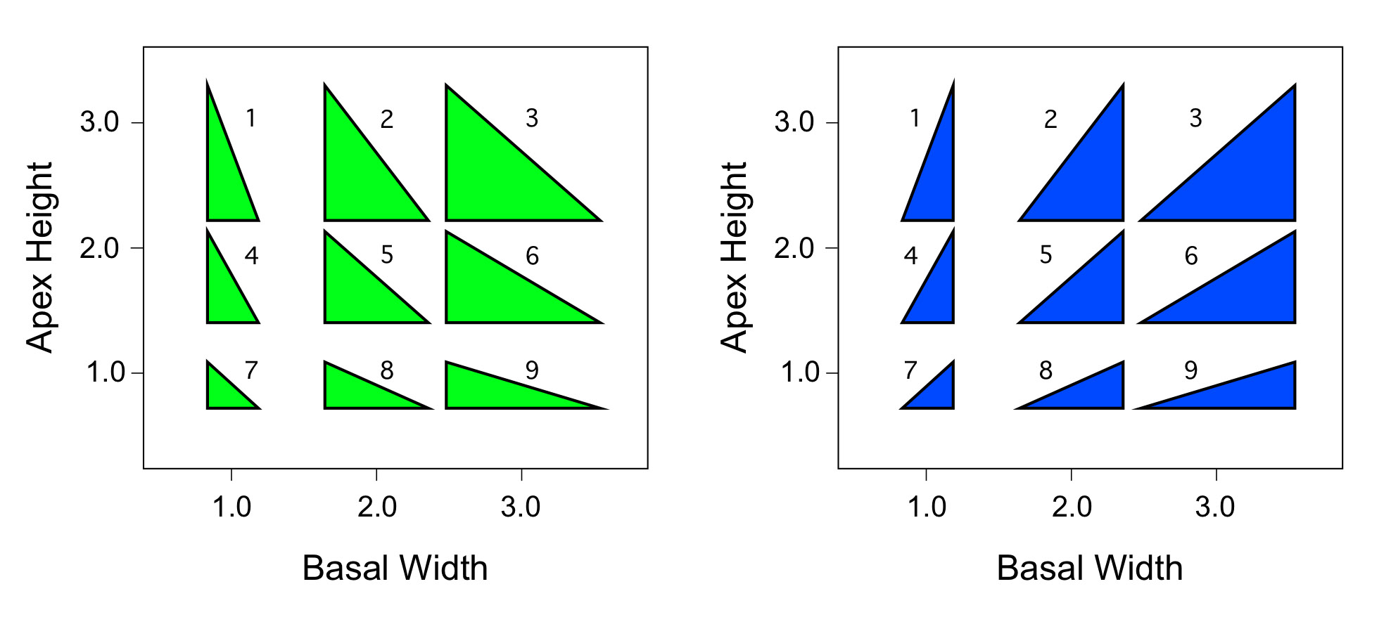
Figure 2. Plot of right triangles with basal width and apex height dimensions equal to those of the isosceles triangles shown in Fig. 1. Note that these triangles, which are clearly different from each other and from the previous set of isosceles triangles, plot in exactly the same positions within the ordination space formed by these two distance variables.
For the example shown in Figure 1 I chose to draw isosceles triangles in the space. I could have chosen any type of triangle. Figure 2 shows the same plot for right triangles that verge either to the left or the right. Of course, right triangles still have a basal width and an apex height. We can use the same variables to describe them. But note that when we do both sets of right triangles plot in exactly the same positions as the set of isosceles triangles in Figure 1.
This simple experiment suggests the geometric space formed by these two distance variables is anything but simple and straightforward to interpret for morphological data. Size and shape are confounded in complex ways and individual positions within the space represent large (effectively infinite) families of possible shapes (in this case triangles), each of which differs from the others in shape, size, or both. Such variables may be able to be used to test simple hypotheses involving shapes whose range of variation is limited (e.g., out example trilobite data). Even in these cases though, the inherent geometric ambiguity of the space formed by such variables should always be kept in mind.
If all this complexity applies to the analysis of two distance variables, imagine the problems associated with both assessing and keeping track of the additional complexities that result from the description of shapes using more than two distance variables! As we have already seen, patterns of variation in such data can be assessed using powerful techniques such as PCA and PCoord. But use of these methods does not improve the power of distance variables themselves to describe shapes adequately. If anything, the correct geometric interpretation of multivariate ordination spaces based on inherently ambiguous distance variables is even more complex than this simple two-variable example for any but the most well-behaved datasets.
What to do? Triangles are simple, two-dimensional figures. There must be a geometric space in which the shape of any triangle can be located uniquely. What we need to do is find this space, develop some insight into what this space looks like, and develop tools that will allow us to use this space to make accurate comparisons between shapes. Let’s try to use the Procrustes tool we developed last time on these triangle data to get our heads around what’s going on.
Recall that, under the Procrustes approach, shapes are those aspects of geometry left over after the factors of form difference attributable to (1) position, (2) scaling, and (3) rotation have all been removed from data consisting of the coordinate locations of comparable landmarks. If we take the set of x,y coordinates for the 27 triangles shown in figures 1 and 2 and calculate their Procrustes superposition on the sample mean shape, the resultant plot of superposed coordinate values looks like Figure 3.
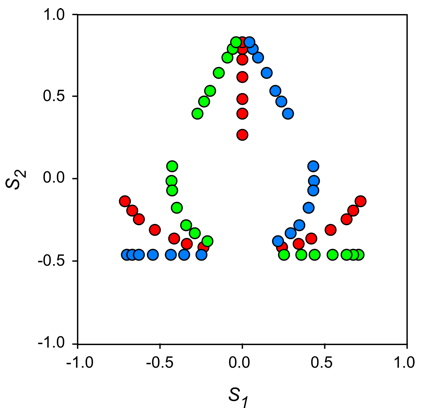
Figure 3. Procrustes superposed shape coordinates for the triangle datasets shown in figs 1 and 2. Color codes as in those figures.
The symmetry of this shape-coordinate plot may come as a surprise. Remember, Procrustes superposition tries to minimize the deviation between a target and a reference form (= the mean shape) at all corresponding landmark locations across the entire form. Sometimes this results in odd-looking rotations of the datasets. But Procrustes superposition has the distinct advantage of minimising shape differences globally.
| Component | Eigenvalue | Shape Variance (%) | Cum. Shape Variance (%) |
|---|---|---|---|
| 1 | 0.058 | 49.88 | 49.88 |
| 2 | 0.057 | 48.64 | 98.52 |
| 3 | 0.002 | 1.48 | 100.00 |
Once these data have been matched for shape variation we can obtain a sense of their linear ordination by performing a standard PCA analysis of the superposed coordinate values. Table 1 provides information about the amount of shape variation that exists in this superposed shape-coordinate dataset. Despite the fact that six variables were used in the analysis, there are only three non-zero eigenvalues. This happens because the Procrustes standardization for position, size, and rotation removes three components of shape variation from a dataset of landmark points described by two Euclidean dimensions. With respect to the remaining axes PC-1 and PC-2 subsume subequal amounts of shape variation with a small remainder being represented on PC-3. Here it is important to emphasize that the three-dimensional representation of the triangle shape space is not a mere by-product of this dataset. Three non-zero eigenvectors would be returned no matter how many triangles were included in the dataset or what their shapes were, so long as they are represented by two-dimensional (x,y) coordinate data matched using the Procrustes method.
Since we have defined shape as that subset of the observed variation left over after standardization for position, size, and rotation, this means that the characteristic shape space for any form represented by three landmarks is three-dimensional. By using appropriate software we can graphically represent the complete mathematical shape space of triangles. Of course, our small dataset of 27 isosceles and right-triangles is but a small subset of all possible triangles. Nevertheless, inspection of this small region of the overall triangle shape space (Fig. 4) yields important insights.
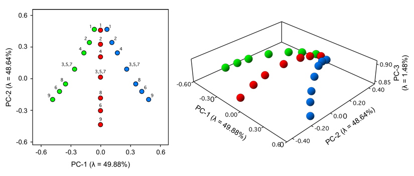
Figure 4. Portion of the overall triangle shape space subsumed by the triangles shown in figs 1 and 2. Plane through the first to principal components of shape variation (left). Perspective diagram of variation along all three shape variation axes (right). Color codes and shape numbers as in previous figures. See text for discussion.
There’s much to discuss with relation to this graph. First, notice that, unlike the distance-based PC space shown in figures 1 and 2, the Procrustes shape space has a unique coordinate location for all three sets of triangles. This means the Procrustes-referenced representation of shape relations is complete. In fact, it’s more complete it probably appears at first glance. Count the number of points in each colour-coded triangle set. That’s odd! There are only seven points in each set. Yet, in figures 1 and 2 there are nine triangles. What happened to the extra two per set?
Recall that in each set the upward-trending diagonal (lower left - upper right) contained forms that differed in size, but not in shape. These forms plotted in different places in the distance-based space because that (traditional) space confounds size and shape relations. Not so the Procrustes space. The fourth point in each series is a coordinate location where three shapes plot. This represents an internal check on the fidelity of the Procrustes shape space. In the distance-based PCA space, shapes that were identical plotted in different locations. In the Procrustes PCA space, these same shapes plot at the same location.
But does the overall picture of shape similarity relations shown in Figure 4 make sense? The triangles in figures 1 and 2 can be subdivided by the upward trending diagonal of identical shapes into two groups. Triangles that plot below the diagonal are wide and low. Those plotting above the diagonal are tall and narrow. Within these subsets the shapes occupying the upper left and lower right corners are more extreme than the two closer to the diagonal. Therefore, we should expect these extreme shapes to represent the ends of each sequence in Figure 4, the identical shapes along the diagonal to represent the middle of each sequence, and the intermediate tall-narrow and short-wide shapes to be located in between, on either side of the group-specific mean shapes (arrows in Fig. 4). This is precisely the ordering of shapes seen in Figure 4.
In terms of inter-group relations, the tall, narrow end-member shapes in each sequence are grouped close together at the top of the diagram because it is possible to bring their landmark locations into close alignment. This correspondence is impossible to achieve with the shorter, broader forms. Therefore, not only is the Procrustes-based shape space portraying shape similarities accurately, it’s also portraying shape differences in a manner that agrees with what would be a taxonomist’s geometric intuition.
The advantages of using the Procrustes alignment as a basis for shape comparison should be clear by now. But there’s more. Perhaps the most intriguing aspect of the Procrustes shape space is the curvature in the shape sequences that’s plainly visible when all three PCA axes are plotted together (Fig. 4, right). It’s almost as though the shapes are lying on the surface of some invisible, underlying structure. As it turns out, that’s exactly the case.
We can better assess the shape of this invisible structure by increasing the sample size and diversity of triangular shapes and repeating the analysis. Figure 5 shows a selection of a dataset of 500 random triangles that were subjected to Procrustes alignment and PCA analysis. Figure 6 details the distribution of these 500 triangles in the space formed by the three PCA axes.
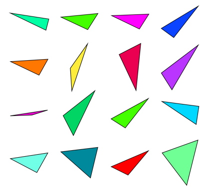
Figure 5. A selection of Procrustes-aligned random triangles used in the exploration of the triangle shape space.
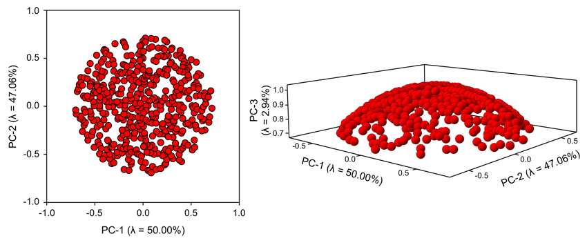
Figure 6. Procrustes PCA ordination of 500 random triangles. See text for discussion.
Because Procrustes shape data are expressed as deviations from a mean shape, the Procrustes PCA space is centred on the mean shape. Also, because dataset is composed of random triangle shapes, the distribution of shapes is roughly circular about the mean shape. However, as you can see from the three-dimensional plot in Figure 6, all the triangle shapes are distributed on the surface of what appears to be a hemispherical form. Regardless of the final geometry of this surface, it would appear Procrustes shape distributions exist in a curved mathematical space.
As it turns out, the full form space for triangles is a perfect sphere. Figure 7 is the canonical representation of this space which, for reasons that will become clear momentarily, we call the pre-shape space.
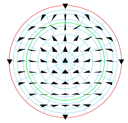
Figure 7. The pre-shape space of triangular forms. Redrawn from Rohlf (http://life.bio.sunysb.edu/morph).
Figure 7 is a two-dimensional map of the three-dimensional triangle pre-shape sphere. Like all spheres, the orientation of the grid system is arbitrary. In this diagram an equilateral triangle, apex up, has been chosen as one pole and the same triangle, apex down as the other pole. The green circle is the sphere’s equator and the lower hemisphere has been folded up to form a ring around the upper hemisphere. Triangles whose apices are located above the baseline are located in the upper hemisphere, those whose apices are located below the baseline in the lower hemisphere. In this orientation the equator represents the set of colinear triangles in which all three vertices lie on the same line.
There are several important things to note about the pre-shape sphere. First, all possible triangles can be mapped to a unique coordinate location on the surface of the sphere. Another way of saying this is that each coordinate location on the pre-shape sphere represents a unique configuration of the three landmarks that make up a triangle. Thus, this sphere’s surface represents a complete representation of the geometry of triangular shape.
What about size? In this representation size is denoted by the radius of the pre-shape sphere. Physically large triangles plot on the surfaces of spheres with large radii, small triangles on spheres with small radii. Recall that, by convention, Procrustes alignment rigidly expands or shrinks all shapes until they have unit centroid size. This operation projects the original shapes—that exist on pre-shape spheres of varying sizes—to their corresponding positions on the unit-sized sphere, thus facilitating direct shape comparison.
What about rotation? Recall that our definition of shape specifically excludes configurations of points that are identical to each other, except for the fact that one has been rotated rigidly relative to the other about their mutual centroid. The pre-shape space is considered ‘pre-shape’ because it places some forms that differ only by rotation at different coordinate locations on the sphere’s surface. This can be appreciated most easily by noting that the equilateral triangles occupying the two polar positions in Figure 7 are identical except for a 180° rotational difference. In fact, the symmetry between the lower and upper hemispheres of the pre-shape sphere arises because of 180° rotational differences (= reflection). However, by correcting for such rotational differences between shapes, the lower hemisphere of the pre-shape space can be mapped onto or merged with the upper hemisphere (or vice versa) thereby achieving a fully realized shape space in which the effects of position, scale, and reflection-rotation have all been removed. Geometrically this transforms the pre-shape sphere into a shape hemisphere. It is this shape hemisphere (also termed the shape half-space) that is being depicted in Figure 6.
Actual shapes that can be characterized by any set of three landmarks represent a realized subset of all possible shapes that map to a particular region on the shape hemisphere. This region may be large or small depending on the amount of shape variation present in the sample. Shapes may be distributed uniformly through the region or arranged in density clusters, again depending on the character of shape variation present in the sample. All the intuitive conceptual conventions we’ve grown accustomed to when thinking about shapes and shape analysis, along with the concepts we use to describe shape variation (e.g., shapes that are similar are ‘close to’ one another, those that are different are ‘distant from’ one another) still apply. But now we understand why in a precise mathematical sense. As a result, this knowledge of what size and shape really are can be used to inform our choice of data-analysis methods and our interpretations of the results of various mathematical operations.
Best of all, these conventions don’t just apply to shapes represented by three landmarks. It’s convenient to work with the triangle shape space because all triangular shapes can be represented in three uncorrelated dimensions we can easily ‘see’ in our mind’s eye and represent on a flat piece of paper or on a computer screen using various graphic conventions. But all shapes that can be described by sets of landmarks have their own shape spaces that behave in precisely the same way.
Morphometricians and topologists call the mathematical surfaces on which shapes reside manifolds, which are mathematical spaces that, on a small enough scale resemble a Euclidean space of a certain dimension. The triangle pre-shape space and the shape hemisphere are both examples of two-dimensional manifolds. The problem with the more complicated manifolds on which shapes defined by more than three landmarks reside is that most of us find it difficult to think in more than three dimensions and our graphic tools for depicting higher dimensional spaces are very primitive. Nevertheless, we can use the triangle shape manifold to gain insight in to the practicalities and complications of truly geometric shape analysis.
At this point I need to make a point about why shape data are different from other sets of data so as not to give you the impression that you can use Procrustes PCA to analyse anything and everything. Recall that PCA (and PCoord, and FA, and MDS) is a generalized data-analysis procedure. It (and they) can be used to analyse data of any sort. The reason why standard distance-based data are not ideally suited for shape data is that, in addition to relations among variables (e.g., covariance, correlation), shape data have an inherent geometry that needs to be respected at the design and computational levels of the analysis. Distance data are simply magnitudes. By themselves they preserve no aspect of the fundamental geometry of the shape. This places constraints on the analysis and interpretation of shape data that simply doesn’t exist for other, more generalized data types.
In a sense standardizing generalized data corrects for the same sorts of factors as the Procrustes standardization for position and size. In some cases it makes sense to standardize data. In others it doesn’t make sense to do so. It almost always makes sense to undertake such standardizations for shape data. But there is no routinely invoked equivalent for rotation to a common reference in non-shape data, The bottom line is, the inherent geometry of shape data means they are different in ways that are not handled well by distance-based variables, but that can be handled by the same sorts of data-analysis procedures we have used throughout our discussion of linear regression and multivariate analysis, provided these shapes are represented by landmarks whose positions relative to one another have been rigidly matched using Procrustes superposition (or an equivalent matching technique).
Let’s end this first exploration of shape theory by discussing a few of the complications that follow from shapes existing mathematically on a curved manifold. If the shape space is curved this means that, strictly speaking, it is inappropriate to use tools of linear algebra (e.g., covariances, eigenanalysis) to explore and summarize relations among shapes. The basic problem is illustrated in Figure 8.
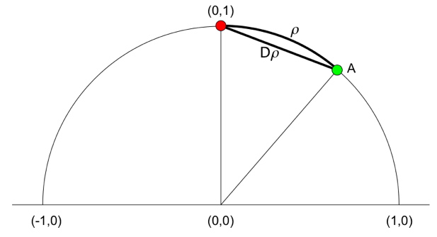
Figure 8. A cross-section through the triangle shape space with the positions of two shapes indicated. See text for discussion.
Since hypotheses about shapes typically turn on the issue of shape similarity, and since shape similarity is quantified by the distance between two shapes or between a shape and the reference shape in the context of the shape space, it is important to calculate the distances, between shapes accurately. The distances we’re interested in are the distances of the shortest curves between two configurations’ coordinate positions along the shape manifold. However, the easiest distances to calculate are the linear distances between points on the manifold. The full, curved distance is termed the Procrustes distance (ρ in Fig. 8) and the linear distance the partial Procrustes distance (Dρ in Fig. 8). As you might imagine, the equations used for calculating the Procrustes distance are formidable, especially when the shape space is high-dimensional. However, we’ve all seen this problem before and are aware of readily available solution.
An important hint at the solution is provided in Figure 7. This is a map of the three-dimensional triangle pre-shape space that’s been flattened out to occupy two dimensions. Note that the method employed to flatten the three-dimensional space has left the points in the lower hemisphere wildly distorted, but points in the upper hemisphere at positions close to their true three-dimensional positions.
I’ve accentuated the difference between ρ and Dρ in Figure 8 by placing the green point (A) a good distance from the reference shape (red point). If, in your mind’s eye, you move the green point along the curve toward the red point a difference between ρ and Dρ remains, but becomes far less marked. Therefore, if our sample of shapes are more-or-less similar to start with, substituting Dρ for ρ should not introduce a large error into estimates, plots, and summaries of shape similarity.
Here it is appropriate to note that landmark datasets are often biased toward overall shape similarity insofar as it is comparatively rare to find sets of organisms with radically different morphologies that can be represented adequately by sets of landmarks. The simple fact that the same set of landmarks must be able to be found on all specimens in the sample goes a long way toward ensuring the the range of shape differences included in any landmark-based analysis is relatively small. For those who like to check assumptions, tests are available to determine how much distortion is likely to be present in Procrustes-based shape analysis. So, we can simplify our problem by taking advantage of linear approaches to data analysis, providing our sample doesn’t encompass too much shape variation.
This having been said, from a practical point-of view the problem of distortion due to inappropriate selection of tangent-plane orientation is usually far more important than distortion due to the range of shape variation present in a sample. In previous discussions you may have wondered why it’s standard for Procrustes superposition to express shape variation as deviation from the mean shape. After all, we don’t usually express distance-based data as a deviation from the mean distance. Moreover, there are other reference forms that could conceivably be used as a reference for a set of shape data (e.g., either the juvenile or mature adult forms in an ontogenetic study, a putative ancestral form in an evolutionary study, a holotypic form in a taxonomic study). What, if anything, is so darn special about the sample mean shape?
The answer to this question has to do not with some stylistic chauvinism among geometric morphometricians, but with the fundamental geometry of the Procrustes shape space. If shape variation in a sample is moderate, it is possible to project shape configuration locations from their positions on the surface of the shape manifold to a linear plane where the well-developed, traditional, and familiar tools of linear algebra can be used to quantify, summarize, represent, and test shape distributions. But there are an infinite number of possible planes that could be used for this purpose. Which, from among this infinite set of tangent planes, is the best choice?
Figure 9 shows two possible tangent plane choices for a dataset composed of two groups, green and blue. In this hypothetical example the shapes exhibited by the green and blue groups are quite distinct. The orientations of the two tangent planes are given by locating tangent points on the Procrustes shape hemisphere. Since each point on that surface corresponds to a configuration of landmark points, this is tantamount to specifying a reference shape. The red dot represents the position of the mean shape for the pooled sample. The yellow dot represents an alternative and arbitrary choice of reference shape. There are several ways of performing the projection, which we’ll discuss in a moment. For now however, let’s assume we’re going to perform a simple, orthogonal or major axis projection to the tangent plane.
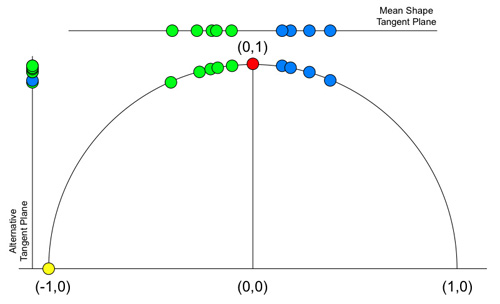
Figure 9. A cross-section through the triangle shape space with the positions of two alternative tangent planes indicated. See text for discussion.
Once we’ve got a clear picture of what the choice of tangent planes entails for the analysis, the correct choice is equally clear. Selecting a point at the periphery of a shape distribution (the yellow point in Fig. 9) guarantees a relatively high level of distortion in the resultant shape ordination due to the curvature of the Procrustes shape space. The effect has been exaggerated in Figure 9 by placing the yellow dot well outside the limits of the observed sample’s shape variation. Nevertheless, and as I hope you can see from the diagram, the distortion will be present for any reference shape choice drawn from the periphery (or beyond) of the shape distribution.
Contrast this with the situation that results from selecting the mean shape (= red dot) as the basis for tangent-plane orientation. This is a position that is guaranteed to orient the tangent plane in a position that minimizes curved-space distortion for the sample. Distortion is present in projections to a tangent plane defined by the mean shape and will be greater for those points at the periphery (as opposed to the centre) of the shape distribution. Some degree of distortion is inevitable whenever a distribution that exists in a high-dimensional space is represented in spaces of lower dimensionality. But as you can see from Figure 9, the amount of distortion is much reduced. For this hypothetical dataset the difference is that of being able to recognize and interpret the shape difference that characterize these groups or not.
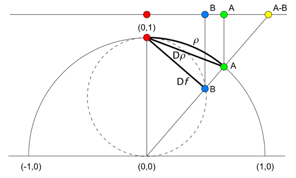
Figure 10. A cross-section through the triangle shape space with the geometry of three alternative tangent plane projection schemes indicated. See text for discussion.
The last shape-space issue we’ll discuss is the strategies available for making projections of points on the surface of the shape hemisphere to the tangent plane. Alternative approaches are summarized in Figure 10.
For completeness I’ve added a second potential shape manifold to this diagram, shown in Figure 10 as the dashed circle inscribed between the origin and reference shape in the Procrustes shape hemisphere. This is the Kendall shape space (or shape manifold), which is formed by relaxing the constraint that all shapes should be adjusted to unit centroid size. As you can see on the diagram, whereas the Procrustes distance (ρ) can be estimated by partial Procrustes distance (Dρ), this is not the shortest distance between the reference shape and a configuration whose form is identical to that of the comparison shape. This shortest distance is represented by Df in Figure 10, which is termed the full Procrustes distance. The difference here is that the blue point (B) does not lie on the unit Procrustes shape manifold. Instead, it resides at a position along the same trajectory from the shape manifold’s origin, but internal to its surface. This is a position in which the configuration’s shape is the same, but the size is slightly smaller.
Application of this ‘relaxed size’ convention produces an alternative shape space that provides a better overall fit of configurations to the reference, but does so at the cost of continually varying the configuration’s size factor in a highly nonlinear manner. Once again, and as I hope you can appreciate from the diagram, for distributions of shapes that are all fairly similar—the typical case in systematics in general—ρ, Dρ, and Df all converge on similar values. Accordingly, in such situations it’s usually acceptable to employ the more easily calculated partial Procrustes distance in representing shape ordinations.
Regardless of this complication over which space is most appropriate to use as a basis for shape comparison, there are two primary ways of projecting points from the shape space(s) to a tangent plane. The stereographic method projects shape configurations from the origin of the Procrustes shape hemisphere (and/or the polar position of the Kendall shape space) through the positions of the geometrically homologous configurations on the surfaces of these two shape spaces to the tangent plane. In Figure 10 this projection is used to place point A-B.
Note that the stereographic method makes no distinction between the Procrustes shape manifold and Kendall shape manifold. Both ways of representing shape project to identical positions on a tangent plane. This is a distinct advantage. The disadvantage of this approach is that the apparent distance between the reference and the projected point is always an overestimate of the true Procrustes distance (ρ), especially for configurations lying at some distance from the reference shape. Indeed, for forms that lie along the equator of the Procrustes shape manifold (= at the pole of the Kendall shape space) no projection is possible as the distance is infinite. However, this is a rarely encountered situation. In the overwhelming majority of cases involving biological shape analysis the estimate is accurate, through the systematic bias to overestimation is always present.
Alternatively projection to the tangent plane may be undertaken in an orthogonal (= major axis) mode using the orientation of the tangent plane as the basis for projection. In Figure 10 orthogonal projections are used to place points A and B on the tangent plane. For this projection strategy the advantages and disadvantages are reversed from those of the stereographic mode. Here, it makes a difference as to whether you choose to match shapes using the Procrustes or Kendall shape spaces. But in either case the projection underestimates the partial Procrustes distance (Dρ) or the full Procrustes distance (Df) respectively, both of which also underestimate the Procrustes distance. As with the stereographic projection, the magnitude of the distortion increases for those configurations that differ markedly from the reference shape. But in no case does the projection lead to an infinite result. Overall, orthogonal projections from the Procrustes shape manifold produce more accurate estimates of the Procrustes and partial Procrustes distances. Unsurprisingly, orthogonal projections from the Kendall shape manifold produce less accurate estimates of the Procrustes and partial Procrustes distances, but better estimates of the full Procrustes distance.
If you’ve made it this far congratulations (and thank you). It might have seemed like a long, hard slog that had little to do with palaeontology per se. Please be assured that my purpose in this essay—and in this column—is not to turn you into mathematicians. Rather, it’s to explain how the tools of mathematics can make us all better palaeontologists and, if truth be told, to lower the level of intimidation most palaeontologists feel toward mathematics. You don’t have to understand the intricacies of non-linear algebra to be able to design and execute a Procrustes shape analysis intelligently, provided you have a firm grasp of the fundamentals. Most importantly though, as Procrustes analysis is arguably the most powerful tool in the quantitative form-analysis kit, and since the basic data of all palaeontology constitutes form, the ability to conduct such analyses should, in my view, be part of every palaeontologist’s training. Besides, once you’ve got a proper guide. it’s not all that hard to understand.
As for software, I really haven’t covered anything in this column that is new in terms of procedures that require access to new software. Most of the algorithms and calculations have been described in previous columns. The triangle examples are included as part of the Palaeo-Math 101-2 spreadsheet so you can see exactly how the figures I’ve used to illustrate this column were obtained. A full analysis of the raw data can also be performed using Jim Rohlf’s tpsRelw program, which is downloadable from his SUNY morphometrics web site (http://life.bio.sunysb.edu/morph). I’ve written several Mathematica routines that were used to perform all the analyses presented herein. These are available free on request. The only procedures that haven’t been covered in algorithmic detail are the routines used for stereoscopic and orthogonal projection to a tangent plane. I need to develop a few additional concepts before I explain how these projections can be accomplished. Accordingly, they will be the subject of a future column.
Finally, references. There really aren’t that many descriptions of this material that have been written to date for non-mathematical audiences. A full mathematical treatment is provided by Mardia and Dryden (1989) and Dryden and Mardia (1998). The canonical conceptual treatment of the concepts involved are covered by Bookstein (1990). A useful, but somewhat overly complex introductory version of this material can be found Zelditch et al. (2004). Finally, a short, but useful discussion is also included in the help section of Rohlf’s tpsRelw program.
