5. PCA, Eigenanalysis & Regression V
Written by Norm MacLeod - The Natural History Museum, London, UK (email: n.macleod@nhm.ac.uk). This article first appeared in the Nº 59 edition of Palaeontology Newsletter.
Principal Components Analysis (PCA)
This time out we’re going to take up a topic I’ve been looking forward to, and dreading, ever since Phil Donoghue invited me to consider writing this column. Principle components analysis (PCA)—or perhaps more correctly, the method of eigenanalysis on which PCA is based—is pre-eminent among the multivariate, numerical-analysis techniques used by palaeontologists to analyze all kinds of data. Both the theoretical and applied PCA literature are vast. Nevertheless, good explanations for a non-mathematical audience are rare; especially explanations that relate PCA to regression analysis (hence the hybrid title of this column) and that provide examples of its use in the context of morphological data analysis. A good discussion of PCA is also made challenging in that a number of the issues we’ve been discussing in previous columns need to be reviewed and combined with new material.
Since this series is meant to focus on practical issues, the first thing to do is set up a problem. In the last column, on multivariate linear regression, we asked how we could use glabellar length and width measurements taken on a selection of trilobites to estimate overall body length of individuals. Our answer, somewhat surprisingly, was that both variables could be combined to yield quite an accurate estimate of individual body length. We also found, somewhat less surprisingly, that the longer measurement (glabella length) was the better, overall, body-length proxy. This data-analysis situation was predicated on a need to make the classic, least-squares distinction between an independent variable (body length) and a set of dependent variables (glabellar length and width).
Now, let’s change this question slightly. Instead of wanting to know how best to estimate one variable in terms of others, suppose we wanted to (1) explore the relations between all three variables simultaneously and (2) use those relations to create new variables with more desirable statistical properties: such that (a) all these new variables are known to be independent of each other, (b) the relative relations between species in the sample are strictly preserved and (c) the geometric relations between the new variables and the old (measured) variables are both constant and easy to interpret in a meaningful, qualitative manner. That’s a tall order, but it’s precisely what is done by PCA. Indeed, PCA gives us this power and much more besides.
| Genus | Body Length (mm) | Glabellar Length (mm) | Glabellar Width (mm) |
|---|---|---|---|
| Acaste | 23.14 | 3.50 | 3.77 |
| Balizoma | 14.32 | 3.97 | 4.08 |
| Calymene | 51.69 | 10.91 | 10.72 |
| Ceraurus | 21.15 | 4.90 | 4.69 |
| Cheirurus | 31.74 | 9.33 | 12.11 |
| Cybantyx | 26.81 | 11.35 | 10.10 |
| Cybeloides | 25.13 | 6.39 | 6.81 |
| Dalmanites | 32.93 | 8.46 | 6.08 |
| Delphion | 21.81 | 6.92 | 9.01 |
| Ormathops | 13.88 | 5.03 | 4.34 |
| Phacopdina | 21.43 | 7.03 | 6.79 |
| Phacops | 27.23 | 5.30 | 8.19 |
| Placopoaria | 38.15 | 9.40 | 8.71 |
| Pricyclopyge | 40.11 | 14.98 | 12.98 |
| Ptychoparia | 62.17 | 12.25 | 8.71 |
| Rhenops | 55.94 | 19.00 | 13.10 |
| Sphaerexochus | 23.31 | 3,84 | 4.60 |
| Toxochasmops | 46.12 | 8.15 | 11.42 |
| Trimerus | 89.43 | 23.18 | 21.52 |
| Zacanthoides | 47.89 | 13.56 | 11.78 |
| Mean | 36.22 | 9.37 | 8.98 |
| Variance | 346.89 | 27.33 | 18.27 |
On to the data. For this discussion we’ll use the same dataset we used in the last column (Table 1). A three-dimensional scatterplot of these data yields Figure 1.
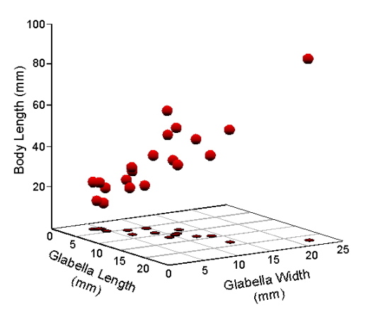
Figure 1. Scatterplot of Table 1 data in a Cartesian coordinate system.
While this is the standard way of representing data consisting of real numbers such as measurements, once you think about it, this Cartesian scatterplot makes an odd assumption about these data. Note the orientation of the three axes. They’re all at right angles to one another—or, at least, they’re supposed to look that way, this being a perspective drawing. In mathematical terms, variable axes drawn this way would be taken to mean these variables are independent in the sense that the pattern of variation among measurements plotted along one variable axis would not be expected to be a good predictor of the pattern of other measurements plotted along another axis. The point is that these data themselves, the plot, and simple logic all tell us body length, glabella length, and glabella width are not independent of one another. We proved that result for this dataset last time.
What is the true relation between these variables? We’ve seen this before, too. The two most common ways to express inter-variable relations is through the covariance or correlation indices. If the variables are all measured in the same units, and if we wish to take the magnitude of the variables into consideration when expressing their relations, we should calculate the covariance between variables (see the Regression 2 column). The structure of covariance relations between multiple variables is usually expressed in terms of the pairwise covariance matrix (Table 2). Here the matrix’s diagonal cells, or ‘trace’, is filled by variable variance values and the off-diagonal cells filled by between-variable covariance values.
| Variable | BL (x1) | GL (x2) | GW (x3) |
|---|---|---|---|
| BL (x1) | 329.549 | 82.832 | 64.995 |
| GL (x2) | 82.832 | 25.966 | 19.299 |
| GW (x3) | 64.995 | 19.299 | 17.353 |
Alternatively, if the variables are measured in different units (e.g., some in mm, some in inches2, some in ml, some in degrees of arc) such that it makes no sense to compare them directly, or if we do not wish to take the magnitude of the variables into consideration when expressing their relations, we should calculate the correlation between them (see the Regression 2 and Regression 4 columns). The structure of correlation relations among multiple variables is usually expressed in terms of the pairwise correlation matrix (Table 3) in which the matrix’s trace is filled by correlations of variables with themselves (= 1.000) and the off-diagonal cells filled by correlations between pairs of different variables
| Variable | BL (x1) | GL (x2) | GW (x3) |
|---|---|---|---|
| BL (x1) | 1.000 | 0.895 | 0.859 |
| GL (x2) | 0.895 | 1.000 | 0.909 |
| GW (x3) | 0.895 | 0.909 | 1.000 |
Note both matrices are symmetrical about their trace.
Now, let’s talk geometry. We can model the distribution of the Table 1 data by enclosing our data points in a volume. The volume that makes the fewest assumptions about the shape of the underlying distribution from which our trilobite sample was drawn is a three-dimensional ellipsoid (Fig. 2).
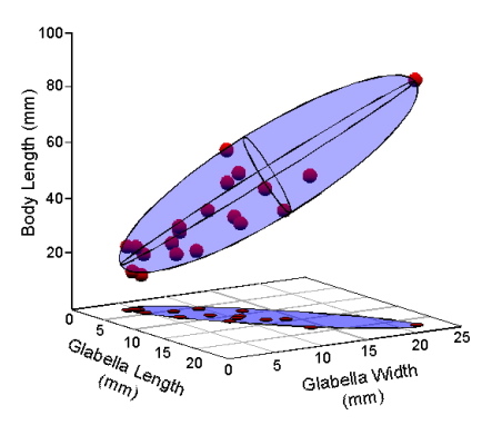
Figure 2. Model of the Table 1 data as a 3-dimensional ellipsoid.
If the three variables exhibited perfect covariance or perfect correlation with one another (e.g., columns 2 and 3 of Table 1 filled with the same values as column 1), the points in Figure 1 would fall along a perfectly straight line oriented at 45° to the three axes. In that case, the ellipse in Figure 2 would collapse to a straight line. By the same token, if the columns of Table 1 were filled with completely random numbers, the points would fill a space best represented by a sphere. The fact that our data represent a somewhat fat cigar shape indicates that their covariance-correlation structure lies somewhere between these two extremes. Observe that the true distribution of our data points in these figures has been systematically distorted because I’ve drawn the body length axis to be approximately the same length as the glabellar length and width axes. Given the interval over which body length values range, this axis really should be four times longer than it is. If I did that, the ellipsoid model would appear much thinner than it’s portrayed. Thus, the true structure of covariance-correlation relations in our trilobite data is closer to being perfect than to being random.
Here’s another way to make the same observation. Take a look at covariance and correlation matrices for those data (tables 2 and 3 respectively). The off-diagonal values are all relatively high, confirming our qualitative geometric intuition. Note also how much easier it is to get a sense of the geometry from looking at the correlation matrix as opposed to the covariance matrix.
In a qualitative sense, what PCA does is to create basic descriptive elements of the model shown in Figure 2. The nature of these descriptive elements is most simply illustrated in two dimensions, which would be analogous to the plot shown at the base of the coordinate systems in figures 1 and 2. Consider the graph of a simple ellipse (Fig. 3).
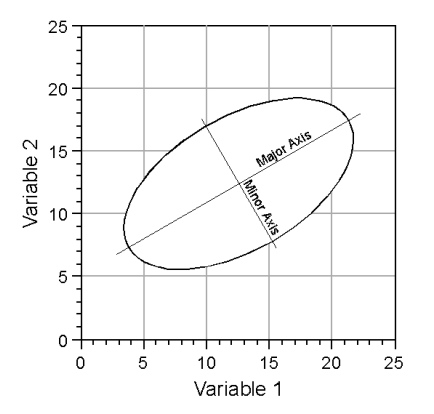
Figure 3. Descriptive elements of an ellipse.
Like a circle—which is a special case of an ellipse— the ellipse’s position is established by its centre. Radiating from this centre are two axes: a long axis typically referred to as the major axis, and a shorter axis typically referred to as a minor axis (also referred to as the semi-major axis or semiaxis). Since these axes are described by two quantities, a length and a direction, they can be represented by vectors. In addition, the most efficient and conventional description of an ellipse requires that the major and minor axes (or vectors) be oriented at right angles to one another. Thus, the model ellipsoid drawn in the space between the three axes of Figure 2 can be characterized by a major axis, oriented along the ellipsoid’s long axis, and two minor axes oriented at right angles both to the major axis and to one another, with each axis being a different length. The mathematical problem inherent in PCA is that of how to take the information embodied by the covariance or the correlation matrix of a sample, and estimate the geometry of ellipsoid model. The hope of PCA is that, by analyzing a sufficiently representative sample you will be able to infer and/or quantify relations existing within the population from which the sample was drawn.
This is both easier and more difficult than it appears. Let’s start off by simplifying our problem even further and only focus on body length and glabella length. We can graph the structure of covariance or the correlation relation directly. For this example we’ll use the correlation matrix so the numbers won’t be so large as to make the underlying geometry unclear. Figure 4A shows this graph. The two vectors represent the correlation between the two variables. One coordinate value represents the correlation of the variable with itself and the other represents its correlation with the other variable. Because the correlation matrix is symmetric, these two vectors are always symmetric about one axis of the ellipsoid model and lie on the same side of the other axis. In addition, because this is a representation of the correlation matrix, the origin of the coordinate system is always the center of the ellipsoid model.
Once we know these quantities it is a relatively simple matter to calculate the model in Figure 4B, at least for the two-variable case. Indeed, we’ve already done this problem back in the Regression 3 column. There, I presented a series of somewhat complex, but tractable formulae that allow you to calculate the slope of a regression line passing through the centroid of a bivariate dataset such that the sum of the deviations of data points from a linear model, measured by distances oriented normal to the linear model, are minimized. That was called Major Axis Regression. The major axis linear regression model is the same thing as the major axis of the PCA ellipsoid model for a bivariate dataset. In this sense then, a PCA of a dataset containing more than two variables is the same as a ‘Major-Axis Multiple-Linear Regression Analysis’.
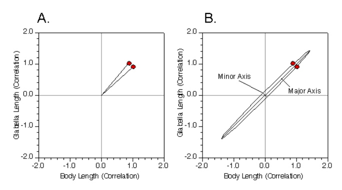
Figure 4. Conceptual diagram of a principal components analysis for two variables. See text for discussion.
OK. That’s the concept bit. Now let’s consider aspects of PCA mathematics. We’ve not going derive PCA from first principles because (1) it’s complex (literally), and (2) it’s unnecessary if you understand the geometric concepts and have access to appropriate software. Nonetheless, there is a bit a terminology and conceptual material associated with the math you do need to understand in order to set up and interpret the results of a PCA correctly.
Fundamental to understanding the math behind PCA is the need to understand that the measurements you make on a specimen can be thought of as terms in an equation that, for the purposes of the analysis, represents the specimen. Take the first three specimens in Table 1. Those specimens are represented by three measurements. For the purposes of a PCA analysis, these measurements may be combined to give the following equations.
Acasta:30.41=23.14+3.50+3.77Balizoma:22.37=14.32+3.97+4.08Calymene:73.32=51.69+10.91+10.72
Geometrically, perhaps the best way to think of equations like these is to consider the three measurements as specifying a vector that represents the object. The basis of PCA is a simple expansion of these equations. If x1 = body length, x2 = glabella length, and x3 = glabella width, the fundamental equations of a three-variable PCA are as follows.
(5.1) a11x1+a12x2+⋯+a1nxn=λx1a21x1+a22x2+⋯+a2nxn=λx2a31x1+a32x2+⋯+a3nxn=λx3⋮an1x1+an2x2+⋯+annxn=λxn
What these equations mean is that there exist a series of coefficients (the alpha-values, think of them as weights) such that when they are multiplied by the object vector in the manner shown, the sums are equal to some constant value (the λ) multiplied by the specimen vectors themselves.
The set of alpha-values are called eigenvectors. These are sets of weight coefficients or ‘loadings’ determined by iterative adjustment of the entire weight-vector system such that, when the first set of eigenvectors are multiplied by the original measurements, the variance of those sums across the entire sample is maximized. Subsequent eigenvectors are adjusted to achieve an identical maximum sum constraint for the residual data. Symmetrical matrixes also yield eigenvectors with the desirable property of being oriented at right angles to one another. In terms of the ellipsoid model described above, the eigenvectors represent the orientations of the major and various minor axes oriented such that they are aligned with the major directions of variation in the sample and are perfectly uncorrelated.
The lambda values are called the ‘eigenvalues’ or the ‘latent roots’. When summed, these roots are equivalent to the maximum variance or correlation uniquely associated with the sample. By convention they are subdivided into component roots assigned to each eigenvector. When the values of all the component eigenvalues are added together they equal the sum of the trace of the basis covariance or correlation matrix. There are as many positive component eigenvalues in a covariance or correlation matrix as there are independent dimensions of variation in these data. Usually, this means there are as many positive eigenvalues as there are measured variables. Symmetrical matrices, such as the covariance and correlation matrices, always produce real-number eigenvalues. Non-symmetric matrices produce complex-number eigenvalues. We don’t want to go there just now. Where we do want to go is to think of the eigenvalues in terms of the ellipsoid model. As a set of constant scalars associated with the eigenvectors and reflecting the amount of variance they represent when combined with the original measurements, the eigenvalues are the lengths of the ellipsoid model's major and set of minor axes.
Decomposition of a covariance, correlation, or any other type of matrix into its eigenvectors and eigenvalues is called eigenanalysis. The basic method used today was developed by Hotelling in the 1930s but, because of the computation-intensive nature of the procedure, it wasn’t often employed for data analysis until the advent of computers. Today, eigenanalysis is applied routinely in fields as disparate as theoretical topology and computer game programming (which, actually, are not as different as you might think). Many of the multivariate methods we’ll be discussing in future columns will make use of eigenanalysis.
Now, on to illustrate these concepts with a few examples. To make the simplest possible illustration of PCA from a geometric point-of-view, let’s continue with the analysis of body length and glabella length described in conceptual terms above. Remember, because that analysis was based on a decomposition correlation matrix we’re not analysing the data presented in Table 1 (above), but rather those variables in their standardized form. Figure 5A plots the values of the two standardized variables while 5B plots these sums of the two PCA equations (see below) for same data in the coordinate space formed by this sample’s two principal component axes. These sums are called the ‘scores’ of the original measurements along the principal component (= eigenvector) variable axes.
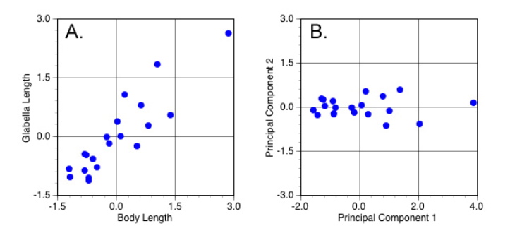
Figure 5. Scatterplots of standardized variables (A) and principal components variables (B) (see text for discussion).
There are several things to notice about this diagram. The most obvious is the alignment of the scores with the PCA plot axes. This alignment means that the PC1 and PC2 (eigen)vectors have been oriented such that their directions coincide with the directions of maximum variation in the original sample. In addition, note this realignment involved a rigid rotation of the original data in the sense that the position of each data point relative to every other data point has been preserved. Points that were close together in Figure 5A remain close together in Figure 5B and vis a vis. Look even more closely and you’ll see another interesting thing about the symmetry between these two graphs. The scores in Figure 5B are not only rotated rigidly from the positions of the original data points in Figure 5A, they’re also reflected about the PC2 axis. The reason for this commonly seen PCA phenomenon is that the direction of the principal component axes (= the eigenvectors) is arbitrary. This reflection is a consequence of the way these axes are calculated and the fact that, from a purely directional point of view, the vector 1, -1 is equivalent to the vector -1, 1. Finally, notice the difference in the scale of the two graphs. The points plotted in Figure 5A range over a little less than 4.5 standard deviation units along both axes. The scores plotted in Figure 5B range over a bit less than 6.0 standard deviation units along PC1, but just a little over 1.0 unit along PC2. This means the scale of the scores along PC1 and PC2 has been adjusted so as to provide a direct reflection the sample variances represented by the associated eigenvectors.
Additional discoveries await inspection of the PCAs numerical results. Equations for the two eigenvectors plotted above are shown below.
PC1=0.707x1+0.707x2
PC2=0.707x1+0.707x2
The numerical values of these equations are the weight coefficients or loadings of each principal component axis. These numbers accomplish everything we just described above. You can also think of these loadings as slopes of the multivariate major axis regression of body length and glabella length on a third variable, PC1 (or PC2) score. Remember, these scores are determined by substituting the values for standardized body length (x1) and standardized glabella length (x2) into these equations and calculating the result for every object in the dataset.
For this sample, the only difference between the PC1 and PC2 equations is a change in the sign of the second loading. This change in sign means the two principal component axes are oriented at right angles to one another. Consequently, the scatterplot shown in Figure 5B is a true representation of the dataset’s inherent geometry, with both axes drawn in their correct relative positions. In contrast, Figure 5A portrays a biased geometry in which the data scatter appears larger than it really is because the Cartesian convention of drawing variable axes at right angles artificially inflates the distal portion of the true coordinate system.
Since the magnitude of the loadings for each variable are identical, the principal component axes lie at an equivalent angle to both the body length and glabella length axes. Because this is a correlation-based PCA, these loadings are the cosines of the angle between the original axis and the principal component axis. Thus, the angle between the body length axis and PC1 is the arccosine (cosine-1) of 0.707, or 45°, a result that accords well with our observations of the data portrayed in Figure 5A.
| Principle Component | Eigenvalue | % Variance | Cum. % Variance |
|---|---|---|---|
| 1 | 1.895 | 94.75 | 94.75 |
| 2 | 0.105 | 5.25 | 100.00 |
Much good information is also contained in the eigenvalue results (Table 5). Recall, the eigenvalues represent the amount of variance assigned to each eigenvector. In the original correlation matrix for these data (Table 3), the variance is given by the sum of the values along the trace. Since this is a correlation matrix, both variables have been standardized to unit variance and the sum of the trace is 2.0. However, even though both standardized body length and standardized glabella length exhibit variances of 1.0, the variance assigned to PC1 is 1.895; almost twice the variance of the original variables. This means that, in terms of between-object contrasts, PC1 represents 94.75 per cent of the information present our sample, with the remaining 5.25 per cent being represented by PC2.
While this result is impressive, it should be taken with a pinch of salt when considering questions of biological interpretation. After all, variance is only one aspect of a dataset and there is no guarantee that dimensions of biological interest will coincide with directions of maximum variance. In making interpretations of PCA results, it also pays to recall the regression-like character of PCA. For any sample, PC1 will always be the axis that represents a factor all individuals have in common. In our example, equality of the PC1 coefficients, and their common positive sign, identify it as an axis of isometric size change (albeit, one calculated from standardized data). In other words, the PCA has uncovered a pronounced tendency within this sample for a unit increase or decrease in standardized body length to be matched by a unit increase or decrease in standardized glabella length. Moreover, this factor, or component, of variation, accounts for almost 95 per cent of the observed variance.
Contrast this with the trend recovered by PC2, in which the coefficients exhibit the same magnitude, but opposite signs. Geometrically, this means there exists a subdominant tendency within this sample for a unit increase or decrease in standardized body length to be matched by a unit decrease or increase in standardized glabella length. This opposing trend is the signature of shape change. Although shape changes account for a relatively minor component of variation in this sample, if the character of shape change is what you’re interested in, PC2 is where you have to go to study it, despite the low variance associated with this shape-change axis. The advantage of a PCA in this context is that, while both size and shape changes are confounded in the original body length and glabella length variables, the principle components representation of these data partitions size changes and shape changes cleanly and convincingly into mutually independent vectors or ‘components’.
This two-variable system is very easy to deal with, so easy that analysis via PCA is a bit of overkill. Principal Component Analysis really comes into its own when analyzing multivariable systems, which is what we’ll do now. For our final example, let’s return to the question posed at the start of the column. This time we’ll eschew geometric simplicity and go whole hog, setting the PCA up so that intrinsic differences in the magnitude of all variables are reflected in the results. This is accomplished by using the covariance matrix calculated from the raw data values as the PCA basis matrix (see Table 2). The sum of the trace of this matrix (392.492) quantifies the overall variance of the sample. Note that, like the correlation matrix (Table 3), the covariance matrix is symmetrical about the trace and so will have real eigenvalues along with eigenvectors oriented normal to one another.
The eigenvectors of this matrix are listed below and the table of eigenvalues below that.
PC1=0.951x1+0.244x2+0.192x3
PC2=0.310x1+0.700x2+0.644x3
PC3=−0.023x1+0.671x2+0.741x3
| Principal Component | Eigenvalue | % Variance | Cum. % Variance |
|---|---|---|---|
| 1 | 383.08 | 97.60 | 97.60 |
| 2 | 7.46 | 1.90 | 99.50 |
| 3 | 2.00 | 0.50 | 100.00 |
As in the previous example, the first eigenvector contains all positive coefficients and so would be commonly interpreted as a size axis. But, this simplistic interpretation—that is to be found throughout the published literature whenever PCA is applied to morphological measurements—is misleading, Note that, contrary to the previous example, the PC1 coefficients are not equal. Since these coefficients express the rate of change in one variable relative to the others (= the slopes of the partial multivariate major axis regressions), this means that, for each unit change in PC1 score, body length change is, on average, much larger than changes in the glabellar measurements. In the previous, two-variable example, we used the term isometric size change to express the pattern of morphological deformation in which all variables increase or decrease in concert and at the same rate. This is the sort of change one sees when a shape drawn on a balloon increases in size as the balloon is blown up or (perhaps more commonly) when we increase the size of a computer graphic while holding the control key down that prevents distortion due to changes in the image’s aspect ratio (Fig. 6). Isometric size change is not the type of morphological change indicated by our three-variable PC1 axis. Rather, along this axis the magnitude of the glabellar measurements is changing at a much slower rate than changes in body length. Moreover, the aspect ratio of the glabella is also changing slightly, as indicated by the difference between the glabellar measurement PC1 coefficients.
In effect, the dominant trend among these three variables is for the glabella of large-sized genera to be slightly narrower along the body axis, and the glabella of small-sized genera to be slightly broader at right angles to the body axis. This is allometric size change (Fig. 6), which is to say size change within which a corresponding shape change is embedded. The condition of allometry is the sort of relation between size and shape change typically seen in biological systems (we’ll discuss why this is so in a future column). Allometric size-shape change also, typically, accounts for the largest single between-object component of variation in morphological datasets. For this sample, allometric size-shape change accounts for more than 97 per cent of the measured variance.
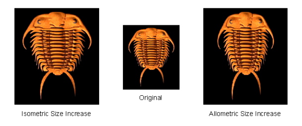
Figure 6. Illustration of the difference between pure or isometric size change and allometric size change, which is accompanied by a change in the specimen's shape.
If quantifying dominant, generalized linear trends within a dataset were all PCA had to offer the palaeontological data analyst it would be well worth the effort. But, as alluded to at the beginning of this column, there’s much more. Let’s move on to an interpretation of PC2. Here we see a contrast between the positive, middle value of the body length loading, and the high negative loadings of the glabellar measurements. The contrast in signs between PC2 and PC1 assures us that the morphological trend represented by the former is uncorrelated with the sample’s allometric size trend. The values of the PC2 loading coefficients show that the second most dominant component of variation in this system is a tendency for individuals with long body lengths to have disproportionately small glabellas. Interpretation of PC3 proceeds in the same way. Once again, the unique pattern of signs assured us that the morphological trend captured by PC3 is uncorrelated with both of the previous principal components. Here, the loading coefficient associated with body length is so small as to be practically negligible. Instead, the equation of this axis reveals a strong contrast between glabellar length and width. Consequently, genera with high scores on PC3 are characterized by a glabella that is strongly elongated in the direction of the body axis.
Since PC2 and PC3 only capture 2.5 per cent of the measured variance, you might suspect that these can be effectively ignored and such may well be the case. In fact, one of the routine uses of PCA is to reduce the dimensionality of a variable system. It is often the case that large number of variables can be reduced to just two or three principal components while still preserving a very high percentage of the measured variation. However, when dealing with so few variables it’s always a good idea to make the most of what you’ve got, even if might turn out not to be significant statistically later on. As a last exercise then, I’ll summarize the distribution of objects in a size-shape space defined by our principal component axes and relate those ordinations to the interpretations I’ve outlined above.
Figures 7A and 7B illustrate the locations of all genera within our three-dimensional principal components system. Note again the similarity of the ordination in Figure 7A to that obtained from the two-variable analysis (Fig. 5B)1. This is due to the relatively small amount of additional variance contributed by glabellar width (see Table 2). To get a sense of the three-dimensional structure of the PCA scores, in your mind’s eye hinge Figure 5B up, out of the plane of the paper about the common axis (PC2) so that it forms a right angled plane with respect to Figure 5A.
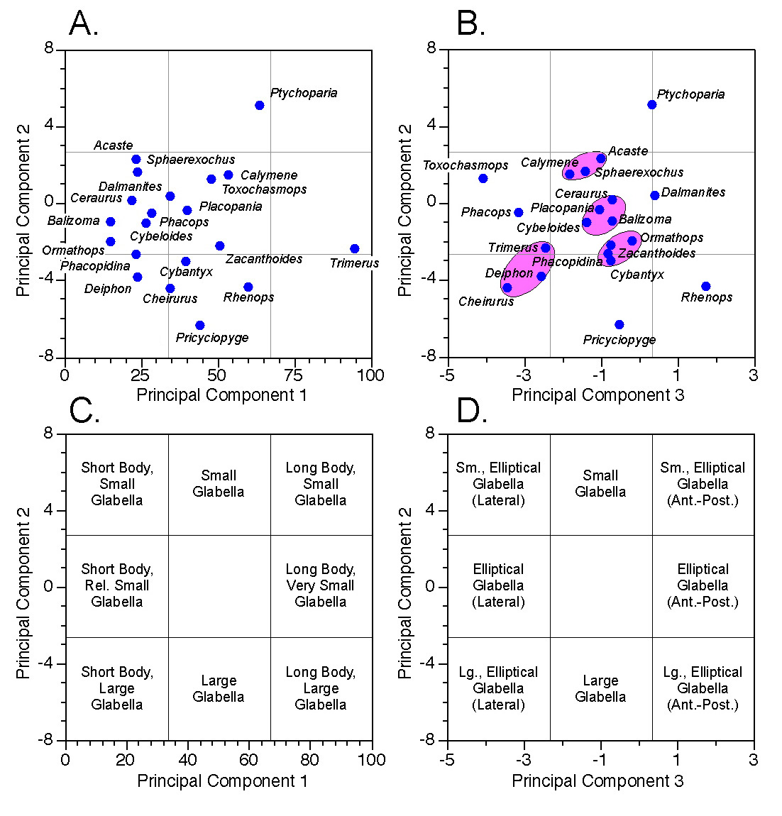
Figure 7. Scatterplots (A-B) and morphological interpretations (C-D) of principal component scores along planes defined by PC-1 and PC-2 (A, C) and PC-2 and PC-3 (B, D). See text for discussion.
Figures 7C and 7D assign relative morphological characteristics to regions of the score scatterplots based on our previous interpretations of the principal component axes. Genera whose projected score positions lie within regions so delimited would be assigned to their corresponding broad morphological categories. Of course, it’s an open question as to whether the specimens I’ve chosen to represent these genera truly are representative. Nevertheless, the analysis could, in principle, be repeated on a larger, more representative sample and these provisional morphological category assignments confirmed or revised. Also note how the score ordinations tend to resolve themselves into subgroups and outliers separated by gaps (some of the more obvious of these are indicated in Fig. 7B). These gaps may reflect consistent and interpretable aspects of the morphological system (e.g., species boundaries, functional constraints) whose morphological character can be inferred from the geometric interpretation of the principal component axes, despite the fact that no specimen representing this morphology was included in the sample.
Principal components analysis—and the eigenanalysis technique upon which it is based—is a powerful data analysis tool. It can be treated as a method in its own right or used as a component part of more complex methods. While PCA is often used as a ‘black box’, the time taken to understand this method’s geometry will be more than repaid in better data analytic designs and better interpretations. All that’s left for me is to close with a few comments about calculating your own PCAs.
Unfortunately, MS-Excel does not provide a routine for determining eigenvalues or eigenvectors within its data analysis library. [Note: The basic eigenvalues and eigenvector results shown in this column’s accompanying spreadsheet were preformed in Mathematica™.] It is possible to programme MS-Excel to perform the necessary calculations, but doing so is not a trivial undertaking. The spreadsheet accompanying this column takes these externally computed eigenvalues and eigenvectors and shows how they can be combined with the original data to yield the PCA scores and plotted in MS-Excel. Those wishing to perform PCA on their data have a variety of options. One can simply obtain a specialized multivariate data analysis package that includes or supports eigenanalysis. Such packages are available as freeware (e.g., PAST) or commercial software (e.g., Statistica™, Systat™, MatLab™, Mathematica™). Alternatively, one can obtain software add-ons to MS-Excel that extend its data analysis toolkit to cover eigenanalysis. There are many of these as well, including freeware (e.g., PopTools) and commercial packages (e.g., XLStat, StatistiXL). New software tools for performing the necessary calculation are also appearing daily on various web search engines. Given this range of alternatives, there is a eigenanalysis/PCA package out there that is right for your needs, computer system, budget, expertise, and level of interest.
The references listed below contain descriptions of principal components analysis I’ve found useful over the years and discuss some of its variants/extensions in more detail than I’ve had an opportunity to do here.
References
CHATFIELD, C. and COLLINS, A. J. 1980. Introduction to multivariate analysis. Chapman and Hall, London, 246 pp.
DAVIS, J. C. 2002. Statistics and data analysis in geology (third edition). John Wiley and Sons, New York, 638 pp.
JACKSON, J. E. 1991. A user's guide to principal components. John Wiley & Sons, New York, 592 pp.
JOLLIFFE, I. T. 2002. Principal component analysis (second edition). Springer-Verlag. New York, 516 pp.
MANLEY, B. F. J. 1994. Multivariate statistical methods: a primer. Chapman & Hall, Bury, St. Edmonds, Suffolk, 215 pp.
SWAN, A. R. H. and SANDILANDS, M. 1995. Introduction to geological data analysis. Blackwell Science, Oxford, 446 pp.
Footnotes
1Don’t be fooled by distortions induced, this time, by drawing the axes to the same physical size, but different scale ranges.
