9. Data Blocks and Partial Least Squares Analysis
Written by Norm MacLeod - The Natural History Museum, London, UK (email: n.macleod@nhm.ac.uk). This article first appeared in the Nº 63 edition of Palaeontology Newsletter.
Introduction
In the last four columns we've looked at problems associated with characterizing and identifying patterns in single datasets. An implicit assumption that runs across all the methods we've discussed so far (bivariate regression, multivariate regression, PCA, Factor Analysis, PCOORD, and correspondence analysis) is that the objects included in the dataset represent independent and randomly selected samples drawn from a population of interest. Using our trilobite dataset as an example, if we are asking questions about this particular assemblage of 20 trilobite genera the results we have obtained to date are perfectly valid. However, it's a big world out there and we'd often like to know how one type of data relates to another type of data. For example, in all but the last of these columns we were concerned with the analysis of simple morphological data. We first considered bivariate data (the linear regression columns), but expanded that to a (still simple) three-variable system when we came to our discussions of the various single-sample multivariate methods. Then, in the last column I wanted to show how another type of data might be handled and so introduced some ecological data in the form of hypothetical frequency counts of these 20 genera in different environments. I'd now like to ask the next most obvious question 'What can we do if we want to explore how the morphological variables relate to the ecological variables for these taxa?'.
As a matter of fact we've already discussed one approach of this situation: what to do if we want to relate one variable to a suite of others. In that case the appropriate approach is multiple regression. Using this method the pattern of linear variation in a dependent variable (e.g., a morphological variable) can be compared to linear patterns of variation in a suite of independent variables (e.g., ecological variables). The purpose of such an analysis would be to (1) assess the overall significance of the various linear relations between the dependent and independent variables and (2) obtain information about the structure of those relations (e.g., which independent variables show the strongest patterns of covariation; which the least). But this method only yields information for one dependent variable at a time. What if we want to assess the significance and structure of covariation for two different multivariate blocks of variables?
There are two approaches for addressing this data analysis situation: canonical correlation analysis (CCA) and partial least squares (PLS) analysis. The former has been around for some time while the latter is something of a new kid on the data-analysis block. I've always found it curious that neither has figured prominently in palaeontological analyses to date, though canonical correlation has been used for many years by ecologists, economists, psychometricians, and a host of others, while PLS made its impact felt first in the field of chemometrics. I think part of the problem has been that CCA requires the algebraic manipulation of complex, non-symmetric matrices that are beyond the capabilities of hand calculators and even simple spreadsheet programmes. Canonical correlation routines are also somewhat rare in various so-called 'canned' computer packages, though they are straightforward to programme in high-level computer languages or using tools such as Mathematica, Maple or MatLab. In this essay, we'll focus on PLS, in part because it's computationally simpler and illustrates many of the same principles as CCA, but mostly because it has several distinct advantages over CCA. Both methods deserve to be used much more widely in palaeontology.
First, let's review our data. You'll remember the trilobite morphological data, three variables measured on a suite of 20 trilobite specimens (Table 9.1).
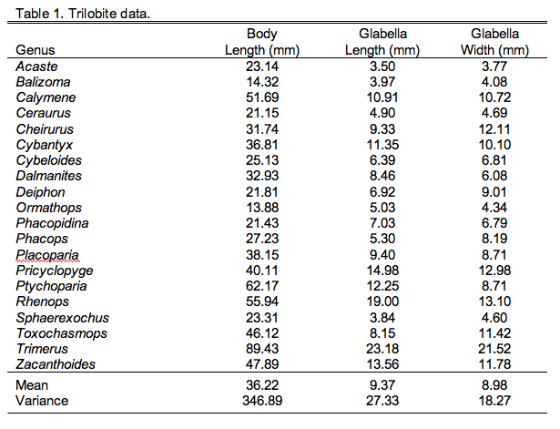
Those following closely will also recall the hypothetical trilobite occurrence frequency data from a suite of seven facies arrayed along a crude onshore-offshore gradient (Table 9.2).
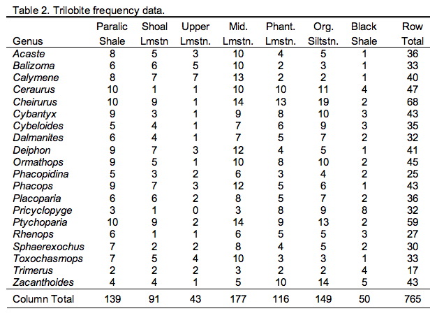
One of the purposes of using the frequency data in our previous discussion of correspondence analysis was to illustrate the superior data handing capabilities of that method. The scaling procedures inherent in correspondence analysis mean essentially any type of data can be submitted to this procedure. Partial least squares analysis is also a generalized descriptive technique and so makes no particular distributional assumptions about the data. Nevertheless, this seems as good a place as any to point out that all descriptive methods work better if the data exhibit some similarity to a normal distribution. Counts are always suspect from a distributional point of view because they typically follow a Poisson distribution (see Fig. 9.1A). Since we'll be making use of the correlation relation in our PLS analysis, and since correlations can be badly biased by outliers, I've transformed the ecological data using a variant of Bartlett's (1936) square-root transformation to make them more normal (Fig. 9.1B). The morphological data were also transformed by taking the log10 of their values since it is well known that this transformation makes variables more linear and removes any correlation between the variance and the mean (see the 'Data Blocks' worksheet of the PalaeoMath 101 spreadsheet for these transformed matrices).
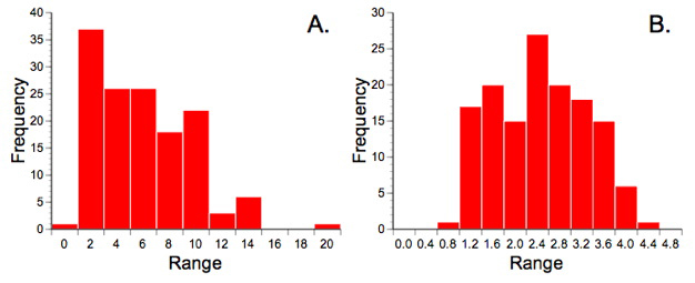
Figure 9.1. Trilobite frequency count data prior to (A) and after (B) transformation by the equation y=sqrtx+0.3, which is variation of the Bartlett (1936) square-root transformation. Note the similarity of A to a Poisson distribution. Strictly speaking the transformation only made these data more normal (as they still do not conform to a normal distribution) but it did improve the balance of the distribution markedly and reduced the number of outlying values.
Now that we have our data in appropriate shape it's time to talk about the comparisons we want to make. PLS has many similarities to PCA, one of which is that you can base the analysis on either the covariance or correlation matrices. For these data the correlation matrix is preferred because the different data groups have different units and characteristically different magnitudes (see the Data Blocks worksheet). As with PCA, you need to consider what basis matrix to use carefully. A covariance matrix is preferred if scaling differences among the variables is something you want the data analysis to take into consideration. For example, if these were two different groups of morphometric variables and one (say the head variables) were characteristically larger than then other (say the tail variables), I might want to include this distinction in the analysis. If I chose to base my PLS analysis on the covariance matrix of raw (though transformed) values, the results would be implicitly weighted toward the larger (= more variable) head variables. On the other hand, if I didn't want these distinctions to affect the results of my analysis I'd want to standardize all my data first so the variances for all variables would be equal, in which case I'd be using a correlation matrix as the basis for my analysis. This standardized covariance, or correlation, matrix for the combined trilobite morphological and ecological variables is shown in Table 9.3.
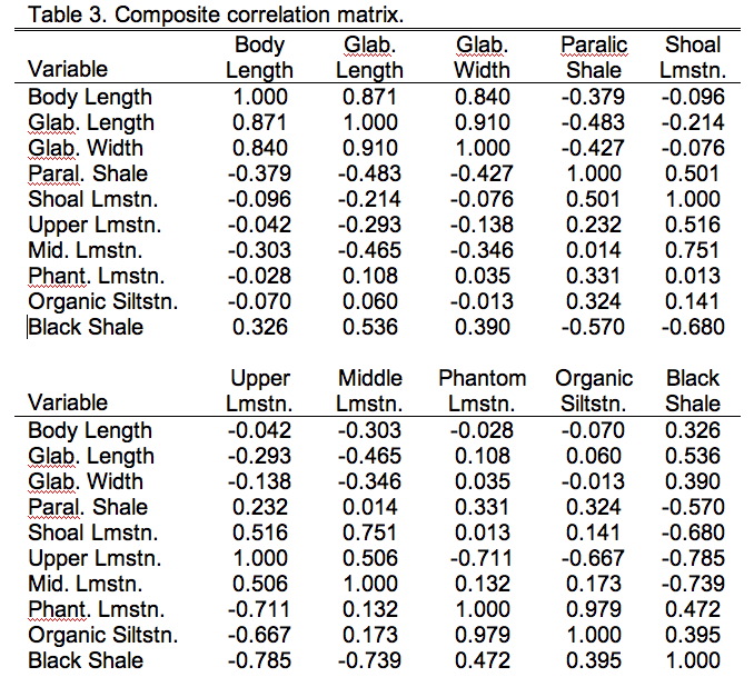
By now you should be familiar with the general form of a correlation matrix (see the PalaeoMath 101 column in Newsletter 58 for a review). The composite matrices we use for PLS analyses are, however, a bit different. On first inspection they might look like perfectly normal correlation matrices. The diagonal is filled with 1's and the upper and lower parts are mirror images of one another. We could analyze the whole matrix and get a perfectly respectable PCA result. The difference, though lies in the fact that we know there are two different blocks of data here—the morphometric variable block and the ecological variable block. We also know that we're only interested in examining the inter-relations between these data blocks. This knowledge changes everything. Diagrammatically we can represent this block-level structure of Table 9.3 as follows.
| R11 | R12 |
| R21 | R22 |
Here R11 refers to the 3×3 data block containing just the three morphological variables, R22 refers to the 7×7 block containing just the seven ecological variables. Both R21 and R21 refer to the block containing the 3×7 (or 7×3) cross-correlation between the morphological and ecological variables with R21 being a simple transposition of R12 (and vice versa). Two-block PLS analysis foregoes all consideration of blocks R11 and R22 in favour of focusing on block R12. In effect, our PLS analysis will be an eigenanalysis of only that part of the basis matrix both groups share. Table 9.4 shows just this section of Table 9.3.

Note this is a different type of matrix from those we've seen before. It's not square because there are many more columns than rows and it's not symmetric because the two halves of the matrix across the diagonal aren't mirror images of one another. Indeed, there isn't even a diagonal to this matrix! Although this is a common type of matrix, we can't use regular eigenanalysis to decompose it into different modes of variation. That method only works on symmetric, square matrices. Never to fear though; methods have been devised to handle this situation. As a matter of fact, you've already been introduced to the primary method for handling this matrix if you read last issue's column. Singular value decomposition (SVD) rescues us again!
Recall last time we used SVD to perform simultaneous Q-mode and R-mode analyses of the square, symmetric, x2 distance matrix we used as the basis for our example correspondence analysis. That proved a convenient way to represent simultaneous ordinations of objects and variables. Recall also that SVD is an implementation of the Ekhart-Young theorem, which states that for any real matrix X, two matrices, V and U, can be found whose minor products are the identity matrix. This means matrices V and U are composed of vectors arranged at right angles to each other. These matrices are scaled to the original data (X) by matrix W, which is a matrix whose diagonal contains a set of terms called 'singular values' with all off-diagonal elements set to zero. These singular values are the square roots of the eigenvalues of both the V and the U matrices, which are identical for all non-zero singular values. Thus,
X=VWU′
Each eigenvalue represents an axis through the data cloud aligned with the major directions of variation. Since there are three morphological variables (p) and seven ecological variables (q) there will only be p non-zero singular values (since p<q). Matrix V contains the R-mode loadings, which are the patterns of weights (covariance basis matrix) or angles (correlation basis matrix) that specify the directional relation between these new axes and the Q-mode variables. Matrix U' is the transpose of the Q-mode saliences (see below). Here's the bit that concerns us today, however. The Ekhart-Young theorem states the relation is true for any matrix of any shape and/or character, not just square, symmetric matrices. Table 5 shows the singular values and eigenvalues of the R12 data block (see Table 9.3).

These were calculated using the PopTools plug-in for Excel (PC version only). As you can see, from a geometric point-of-view, this cross-variable matrix is highly elongate with very small minor axes. But remember, this is only one block of the overall matrix. Since this is a correlation matrix, we know its total variance is the sum of the number of morphological and ecological variables (p+q=10). Thus, this data block—or more correctly, the cross-variable substructure of the overall correlation matrix—accounts for only 17.56 percent of the total variance. Nevertheless, this is the substructure in which we are interested.
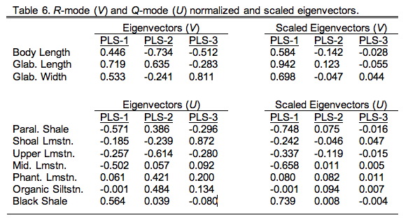
For our example analysis the directional vectors are given in Table 9.6 in their normalized (left) and scaled (right) forms. The normalized form is the most convenient for interpretation as the squares of the values always add up to 1.00. The scaled form is calculated by multiplying the normalized vector coefficients by the appropriate singular value. This operation restores the differences between the scale of the vectors.
These vectors look superficially like principal components, but there's an important difference. Whereas the coefficients or 'loadings' of principal component eigenvectors represent the angular relation between the principal component axes and the original variables, the coefficients of a PLS analysis represent the angular relations of the variables within one data block with respect to those in the other data block. In a sense they represent the variables that are most useful or salient for predicting patterns in the other data block. For this reason they are referred to as saliences.
Turning to an interpretation of these data we first need to ask ourselves how many singular values to interpret. We can approach this using the various qualitative methods discussed in the column on PCA (see the Palaeo-Math 101 column in Newsletter 58) or we can use a more sophisticated, quantitative approach that is has been developed recently for use in generalized multivariate analysis (see Morrison 2004, Zelditch et al. 2004).
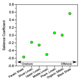
Figure 9.2. Plot of salience coefficients for the environmental hypothetical variables used in the example analysis. While the trend in these data does not conform strictly to an onshore-offshore gradient, and is not strictly linear, there is a strong suggestion that depth-shoreline proximity is an important source of structure in the R12 block of the correlation matrix. This pattern is associated with strong and uniformly positive salience coefficients for the morphological variables (see Table 6) indicating that this depth-shoreline proximity factor is associated morphologically with an allometric size gradient. See text for discussion.
The strength of the relation between the morphological and environmental variables can also be assessed through a simple graphical device. Since we have the R-mode and Q-mode vector for the cross-variable data block we can calculate the R-mode and Q-mode scores in a manner identical to that for PCA. Table 9.7 shows these scores while Figure 9.3 plots them in a simple bivariate ordination space.
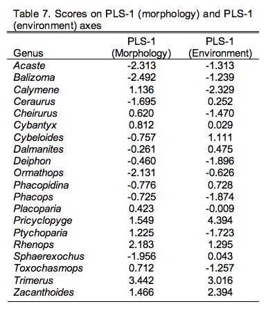
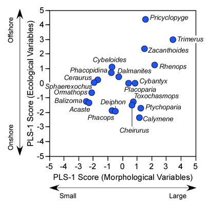
Figure 9.3. Scatterplot of PLS-1 (morphological variables) and PLS-1 (environmental variables) scores for example PLS analysis. This plot represents 97.69% of the correlation structure within the R12 data block.
Comparison of the ordination shown in Figure 3 confirms our interpretation of these results based on the V and U salience matrices. Note large-sized genera (e.g., Trimerus, Zacanthoides, Pricyclopyge, see Table 1) plot toward the upper end of PLS-1 (morphological variables) axis and small-sized genera (e.g., Acaste, Balizoma, Ormathops) toward the lower end, confirming that this axis expresses a generalized size gradient. Moreover, these two groups of genera also display strikingly different environmental occurrence patterns along the PLS-1 (ecological variables) axis with the larger-sized forms being differentially abundant in deep-water facies (see Table 2) and smaller-sized forms preferring shallow-water facies. The linear correlation between the two PLS-1 scores is 0.445, which is just significant statistically for this sample (rcrit.,d.f.=19,a=0.05=0.433) . Based on these results I wouldn't necessarily conclude that size-environment link represents the whole biological story for these data (e.g., the shallow water fauna is composed of mixed small and intermediated sized genera), but this is the strongest, single, linear signal in these data. More importantly for the purposes of this column, by using two-block PLS we've managed to examine the inter-relations between two datasets we've had to treat either separately or as parts of a larger analysis up to this point, and in doing this we've discovered a new patterns in these data that had been hiding there all along.
Partial least squares analysis represents a very powerful and completely generalized approach to ordination and statistical hypothesis testing. Based on a form of PCA, it extends multiple regression analysis, complements canonical correlation analysis, and allows users to test hypotheses about the inter-relations between blocks of observations made on the same objects. Unlike standard PCA which can use a variety of algorithmic approaches to obtain the eigenvalues and eigenvectors of a square, symmetric basis matrix, PLS employs singular value decomposition to obtain the singular values (square roots of eigenvalues) and eigenvectors of parts of PCA basis matrices which may or may not be square, and which will not be symmetric. Aside from the matrix of singular values, this procedure produces two sets of eigenvectors that express the orientational relations between the variables grouped by data blocks: occupying the rows and columns of the basis matrix block. The number of vectors with nonzero lengths will be equivalent to the number of basis-matrix rows (p) or columns (q), whichever is least. In the example above we employed the correlation matrix as the basis for our PLS analysis because of the nature of the variables. PLS can be performed equally well on either covariance or distance matrices.
Unlike standard multiple regression analysis in which a single dependent variable is regressed against a set of independent variables using a linear least-squares minimization criterion (see the PalaeoMath 101 column in Newsletter 55 for a review of linear least-squares minimization), PLS regresses two sets of multiple variables against one another using a major axis minimization (see the PalaeoMath 101 column in Newsletter 57 for a review of linear major axis minimization). Also, the regression coefficients (= slopes) are partial regression coefficients that represent the relation between the trend of the dependent variable and each of the independent variables when the affects of the other independent variables are held constant. Thus, if a pair of variables is highly covariant or correlated, the covariations or correlations of other pairs of variables will be correspondingly reduced since there will not be much residual covariance or correlation structure left after the effects of the first pair are held constant. In contrast, the PLS salience coefficients all represent angular relations with the complete, block-specific, covariance-correlation structure. This makes the interpretation of these coefficients less complex.
Finally, unlike CCA, which recognizes the same block structure as PLS but uses information from all blocks to create a scaled or pooled covariance-correlation basis matrix for SVD decomposition, PLS decomposes only that block which expresses the inter-relations between the variable sets. This means that PLS can focus on only the inter-block aspect of the covariance-correlation substructure irrespective of whether that substructure accounts for a large or small component of the overall covariance-correlation superstructure. Since the coefficients of a CCA, like those of PLS, are used to quantify the inter-relations between blocks of variables, both are referred to as saliences. It is important to note, however, that CCA saliences are equivalent to partial regression coefficients (see above) whereas PLS saliences are analogous to PCA loadings. In effect, CCA represents an attempt to define a set of canonical variables (= linear combinations of variables) for each data block that exhibit overall covariances-correlations that are as large as possible. Indeed, a CCA analysis in which either the set of basis matrix rows or columns contains a single variable is analogous to a major axis-based multiple regression analysis. The goal of PLS differs insofar as it tries to provide a more focused assessment of the inter-block substructure and doesn't allow within-block patterns of covariance-correlation to influence that result.
Partial least squares analysis supports a very large set of investigation types that are often encountered in palaeontological data analysis situations. The example above represents a simple situation in which a set of morphological variables are related to a set of ecological variables, allowing the morphological correlates of ecological distributions (and vice versa) to be assessed. A PLS approach could also be used to investigate inter-relations between different blocks of morphological variables, say from the anterior or posterior regions of a species (e.g., Zelditch et al. 2004) or between different regions of the same morphological structure. This type of study falls within the general 'morphological integration' research programme that tries to identify regions of correlated morphological variation within organismal Baupläne (see Olson and Miller 1958 for a classical treatment of this topic) and is related to the current interest in identifying developmental modules (see Schlosser and Wager 2004). A PLS approach could also be used to examine inter-relations between different types of ecological variables (e.g., organismal-based vs. physio-chemical), or to explore the morphological correlates of genetic variation. The possibilities are virtually endless (see Rychlik et al. 2006 for an good recent example of PLS analysis being used in a systematic context).
As for the practical matter of how to perform your own PLS analysis, unfortunately the choices here are somewhat more limited than for the other methods we've discussed to date. Of course, the PalaeoMath 101 spreadsheet contains the complete calculations for the example PLS analysis presented above. These were performed using the PopTools plug-in for the SVD calculations, but all other calculations were made using the standard MS-Excel data analysis tools. As I mentioned above, generalized mathematical packages (e.g., Mathematica, Maple, MatLab) can also be used to program your own routines. Program systems that perform PLS analysis are somewhat rare, reflecting the method's relatively recent introduction. Of these your best bets at the moment are XL-Stat (some limited PLS capability) and NT-SYS. Since PLS has a longer history of use in chemometrics some stand-alone software is available in programme packages that have been developed for that community. Of these Solo is one of the more complete and better known.
References (cited in the text as well as recommended review articles)
Bartlett, M. S. 1936. The square root transformation in analysis of variance. Journal of the Royal Statistical Society, Supplement, 3, 68-78.
Bookstein, F. L. 1991. Morphometric tools for landmark data: geometry and biology. Cambridge University Press, Cambridge, 435 pp.
Golub, G. H. and Reinsch, C. 1971. Singular value decomposition and lest squares solutions, 134-151. In Wilkinson, J. H. and Reinsch, C., eds). Linear algebra: computer methods for mathematical computation, v. 2. Springer-Verlag, Berlin.
Jackson, J. E. 1991. A user's guide to principal components. John Wiley & Sons, New York, 592 pp.
Morrison, D. F. 2005. Multivariate statistical methods. Duxbury Press, New York, 498 pp.
Olson, E. and Miller, R. 1958. Morphological integration. University of Chicago Press, Chi-cago, 317 pp.
Rychlik, L., Ramalhino, G., and Polly, P. D. 2006. Response to environmental factors and competition: skull, mandible and tooth shapes in Polish water shrews (Neomys, Soricidae, Mammalia). Journal of the Zoological Society, 44(4), 339-351.
Rohlf, F. J. and Corti, M. 2000. Use of partial least squares to study covariation in shape. Systematic Biology, 49(4), 740-753.
Schlosser, G. and Wagner, G. 2004. Modularity in development and evolution. University of Chicago Press, Chicago, 600 pp.
Zelditch, M. L., Swiderski, D. L., Sheets, H. D., and Fink, W. L. 2004. Geometric morphomet-rics for biologists: a primer. Elsevier/Academic Press, Amsterdam, 443 pp.
